[Blog Reivew] Diffusion Meets Flow Matching: Two Sides of the Same Coin

Blog post [Link]
Ruiqi Gao, Emiel Hoogeboom, Jonathan Heek, Valentin De Bortoli, Kevin P. Murphy, Tim Salimans
Google DeepMind
Dec. 2, 2024

Flow matching과 diffusion model을 잘 정리해놓은 포스트가 있어서 정리합니다!

TL;DR

Gaussian Flow matching and Diffusion models are the same!

1. Intro…

최근 Flow matching은 formulation이 간단하고, sampling trajectory의 “straightness”로 많은 인기가 있습니다. 여기서 흔히 하는 질문은,,,

“Which is better, diffusion or flow matching?”

이 포스팅에서 확인하겠지만, diffusion models과 flow matching은 동일하므로, 위 질문은 사실 말이 안되는 것이죠.

이 두 개의 framework가 같다는 것이 그러면 왜 중요할까요? 이는 두 framework의 기법을 같이 사용할 수 있기 때문입니다. (e.g. , flow matching으로 학습한 모델을 deterministic(기존)하지 않고, stochastic sampling을 이용)

이 포스팅에서는 optimal transport path (rectified flow, stochastic interpolants와 관련)에 초점을 맞춰 설명합니다.

2. Overview

Diffusion models

Diffusion process는 이미지를 시간에 따라 점차적으로 Gaussian nosie를 섞으며 noisy하게 만듭니다.

\[{\bf z}_t = \alpha_t {\bf x} + \sigma_t {\boldsymbol \epsilon}, \;\mathrm{where} \; {\boldsymbol \epsilon} \sim \mathcal{N}(0, {\bf I}).\]

\(\alpha_t\)와 \(\sigma_t\)는 noise shedule에 따라 정의되며, \(\alpha_t^2 + \sigma_t^2 = 1\)을 만족하는 경우, variance-preserving이라 합니다.

Sampling (Generating) 과정은 forward process를 “reverse”하는 방식으로 이루어집니다. Gaussian noise로부터, neural network(diffusion model)을 이용해 현재 time step \(t\)에서 노이즈가 제거된 이미지를 예측합니다.

\[{\bf z}_{s} = \alpha_{s} \hat{\bf x} + \sigma_{s} \hat{\boldsymbol \epsilon} \\ \text{where, }\hat{\boldsymbol \epsilon} = ({\bf z}_t - \alpha_t \hat{\bf x}) / \sigma_t\]

이런 sampling 방법은 DDIM이며, Sample의 randomness는 오직 initial Gaussian noise입니다. 즉 전체 reverse process가 deterministic 합니다.

Flow matching

Flow matching에서는 forward process를 data \(\bf x\)와 noise \(\epsilon\)의 linear combination으로 봅니다. (noise가 Gaussian, \(\alpha_t = 1-t, \sigma_t = t\)이라면 diffusion의 forward process와 같습니다.)

\[{\bf z}_t = (1-t) {\bf x} + t {\boldsymbol \epsilon}.\\\]

간단한 대수적 연산을 통해 다음을 유도할 수 있습니다.

\[{\bf z}_t = {\bf z}_{s} + \color{red}{\bf u} \color{black} \cdot (t - s) \text{, for } s < t \text{, where } \color{red}{\bf u} = {\boldsymbol \epsilon} - {\bf x}\]

여기서 \({\bf u}\)는 “velocity”, “flow” 등으로 불립니다.

따라서 given \({\bf z}_t\) 에서 \({\bf z}_s\)를 sampling하기 위해서는 time을 역으로 돌리고, vector field를 최적 추정값 \(\color{blue}{\hat{\bf u}} =\hat{\bf u}({\bf z}_t; t) = \hat{\boldsymbol \epsilon} - \hat{\bf x}\)으로 대체합니다.

\[{\bf z}_{s} = {\bf z}_t + \color{blue}{\hat{\bf u}}\color{black}{\cdot (s - t).}\]

수식이 많아서 중간에 정리를 하자면…

1. Same forward process : 특정 조건하에서 forward process가 동일합니다. (Flow matching의 한쪽 끝이 Gaussian, Diffusion model의 noise schedule이 특정 형태를 가지면)
2. “Similar” sampling process : 두 방법 모두 현재 time step에서 noise가 제거된 clean data를 추정하고, 반복적으로 업데이트 합니다. (Spoiler! 사실 sampling도 동일합니다.)

3. Sampling

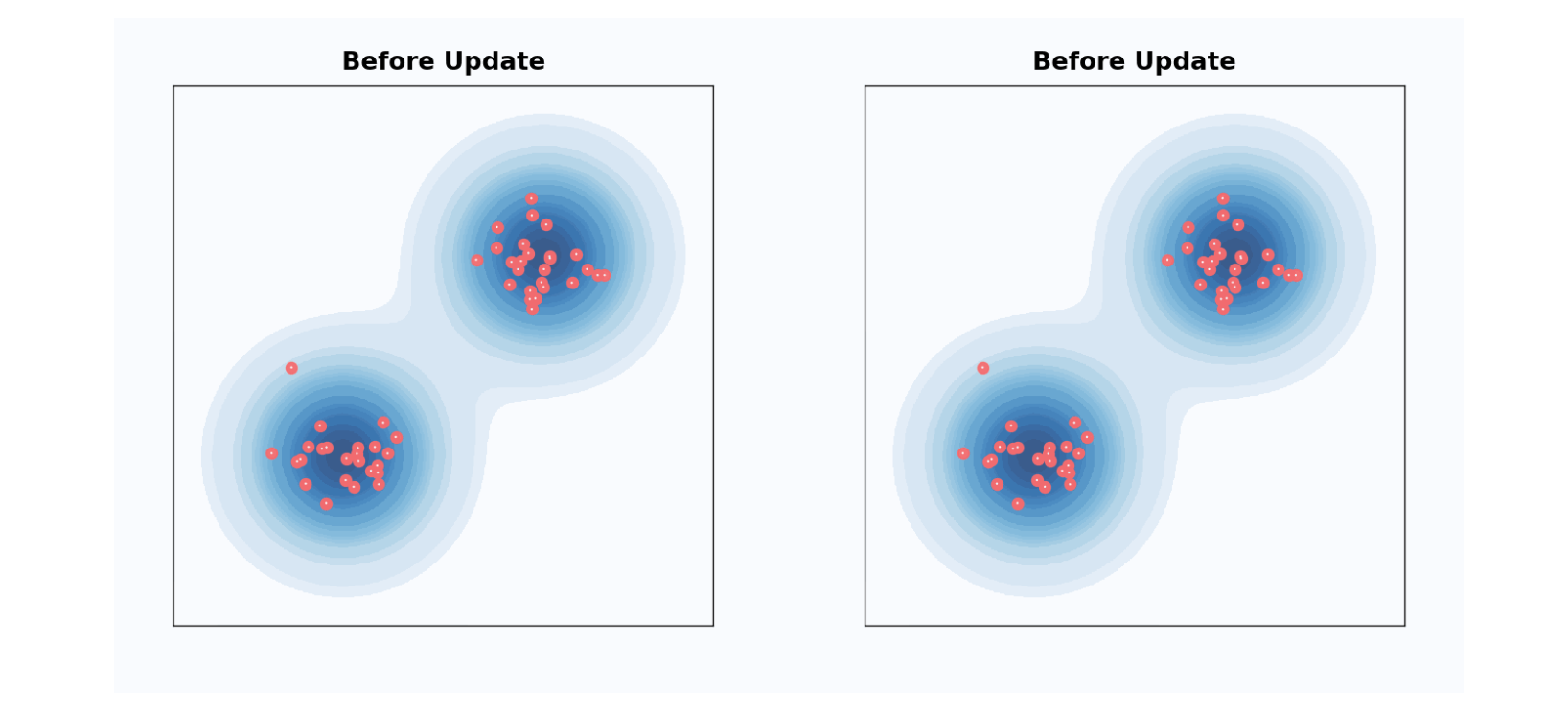
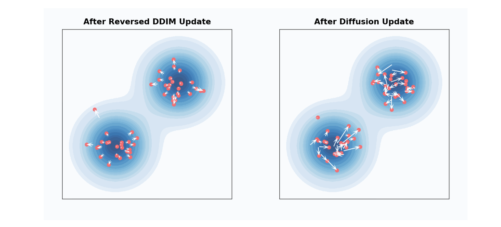
흔히들 flow matching은 “straight” path를 따라 deterministic하고, diffusion model은 “curved” path를 따라 stochastic하다고 생각하지만 이는 잘못된 concept이라고 합니다.

학습된 denoiser 모델을 이용해 random noise를 data로 변환하고 싶다고 가정해봅시다. 위에서 본 것처럼, DDIM은 다음과 같이 주어집니다.

\[{\bf z}_{s} = \alpha_{s} \hat{\bf x} + \sigma_{s} \hat{\boldsymbol \epsilon}\]

이를 rearranging하면 다음과 같은 식으로 표현할 수 있습니다.

\[\tilde{\bf z}_{s} = \tilde{\bf z}_{t} + \mathrm{Network \; output} \cdot (\eta_s - \eta_t)\]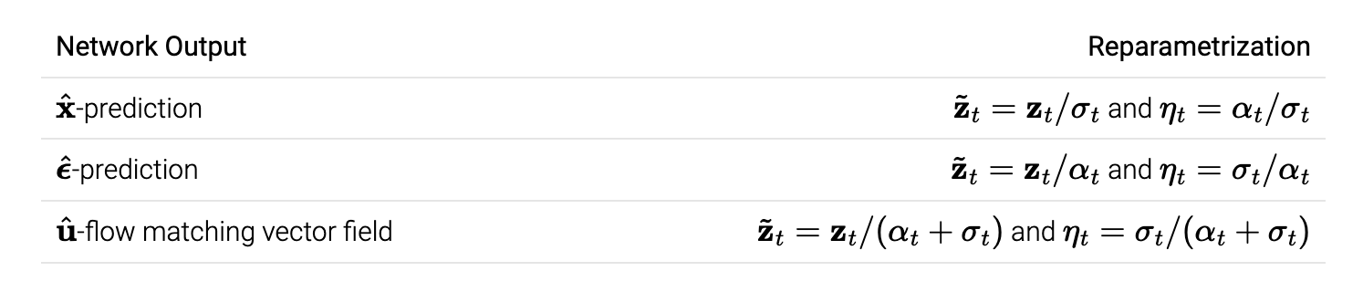

이러고 나니,, flow matching의 식과 비슷하군요. 조금더 형식적으로는, flow matching update가 sampling ODE의 discretized Euler integration (i.e. \(\mathrm{d}{\bf z}_t = \hat{\bf u} \mathrm{d}t\))

Diffusion with DDIM sampler == Flow matching sampler (Euler).

DDIM sampler에 대한 추가 코멘트:

1. (network의 output이 시간에 따라 constant 할 때) DDIM 샘플러는 ODE를 “analytically” 적분합니다. 물론 network의 output은 constant가 아니지만, 이는 DDIM sampler의 부정확성은 ODE의 intractable 적분을 근사하는 데서만 발생함을 의미합니다. DDIM sampler는 Sampling ODE의 discretized Euler integration으로 볼 수 있다고 합니다. \(\mathrm{d}\tilde{\bf z}_t = \mathrm{[Network \; output]}\cdot\mathrm{d}\eta_t\) -> 동일한 update rule

2. DDIM sampler는 \(\alpha_t, \sigma_t\)의 linear scaling에 “invariant”합니다. 이는 scaling이 \(\tilde{\bf z}_t, \eta_t\)에 영향을 못 미치기 때문이라고 합니다.

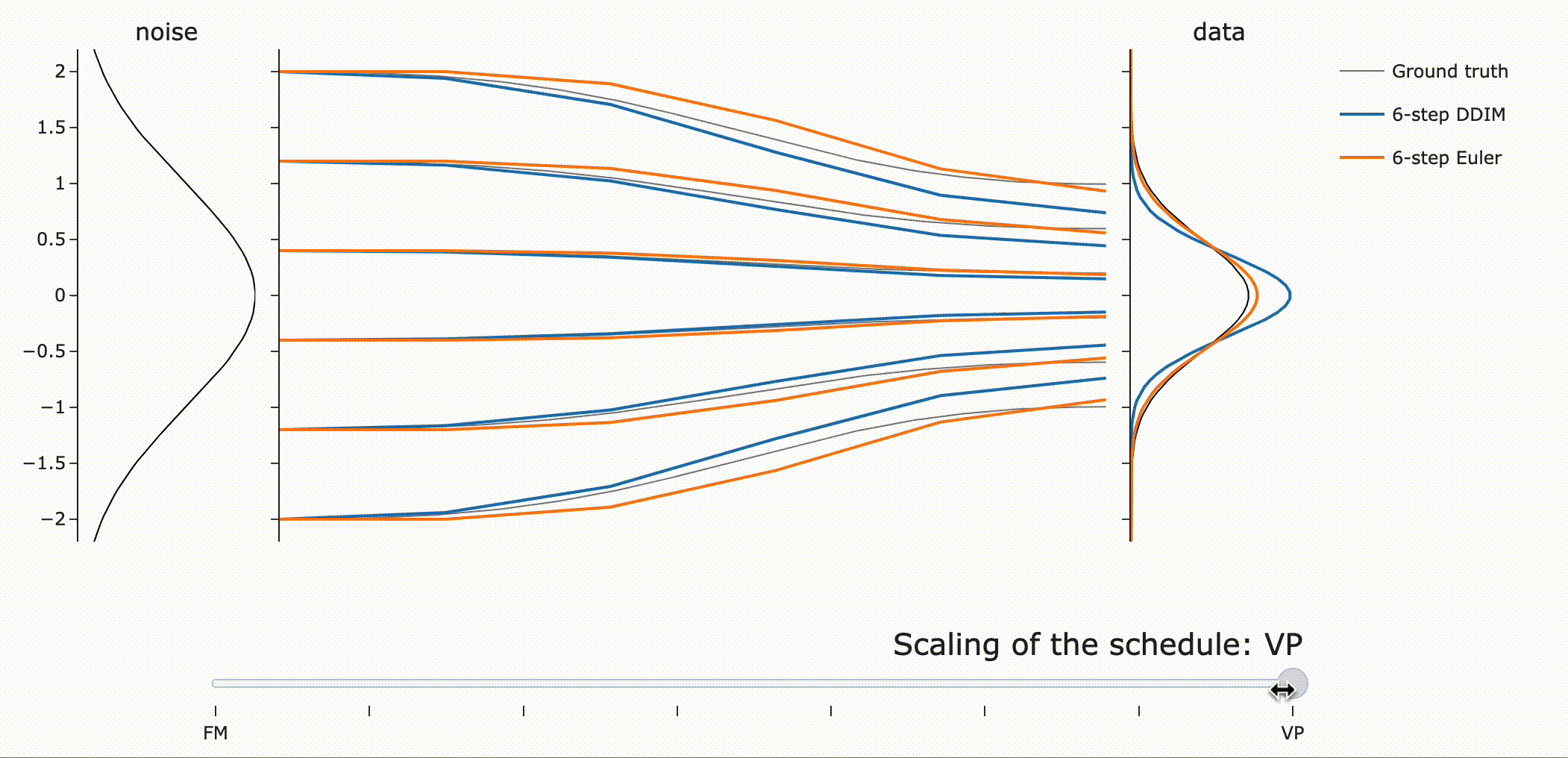
이를 실험적으로 검증하면 다음과 같습니다. (FM : Flow Matching, VP: Variance Preserving)

1. DDIM은 같은 scaling에 관계없이 final data sample을 갖는 것을 확인할 수 있습니다 (파란색). 하지만 \({\bf z}\)는 scale-dependent하므로 path가 달라지는 것을 볼 수 있습니다.

2. Flow ODE Euler sampler는 path, final sample 모두 달라짐!

사람들이 종종 flow matching은 “straight” path를 갖는다고 말하는데 왜 위 Figure는 “curved” 되었을까요?!

만약 모델이 이동하고자 하는 데이터 포인트에 대해 완벽히 확신(confident)한다면, 흐름 매칭 노이즈 스케줄을 사용하여 노이즈에서 데이터로 가는 경로는 직선이 될 것입니다. 직선 경로를 따르는 ODE는 통합 오차(integration error)가 전혀 없다는 점에서 이상적입니다.

그러나, 실제 예측은 단일 포인트가 아니라 더 넓은 분포에 대한 평균입니다. 따라서 “straight to a point”은 “straight to a distribution”과 같지 않습니다.

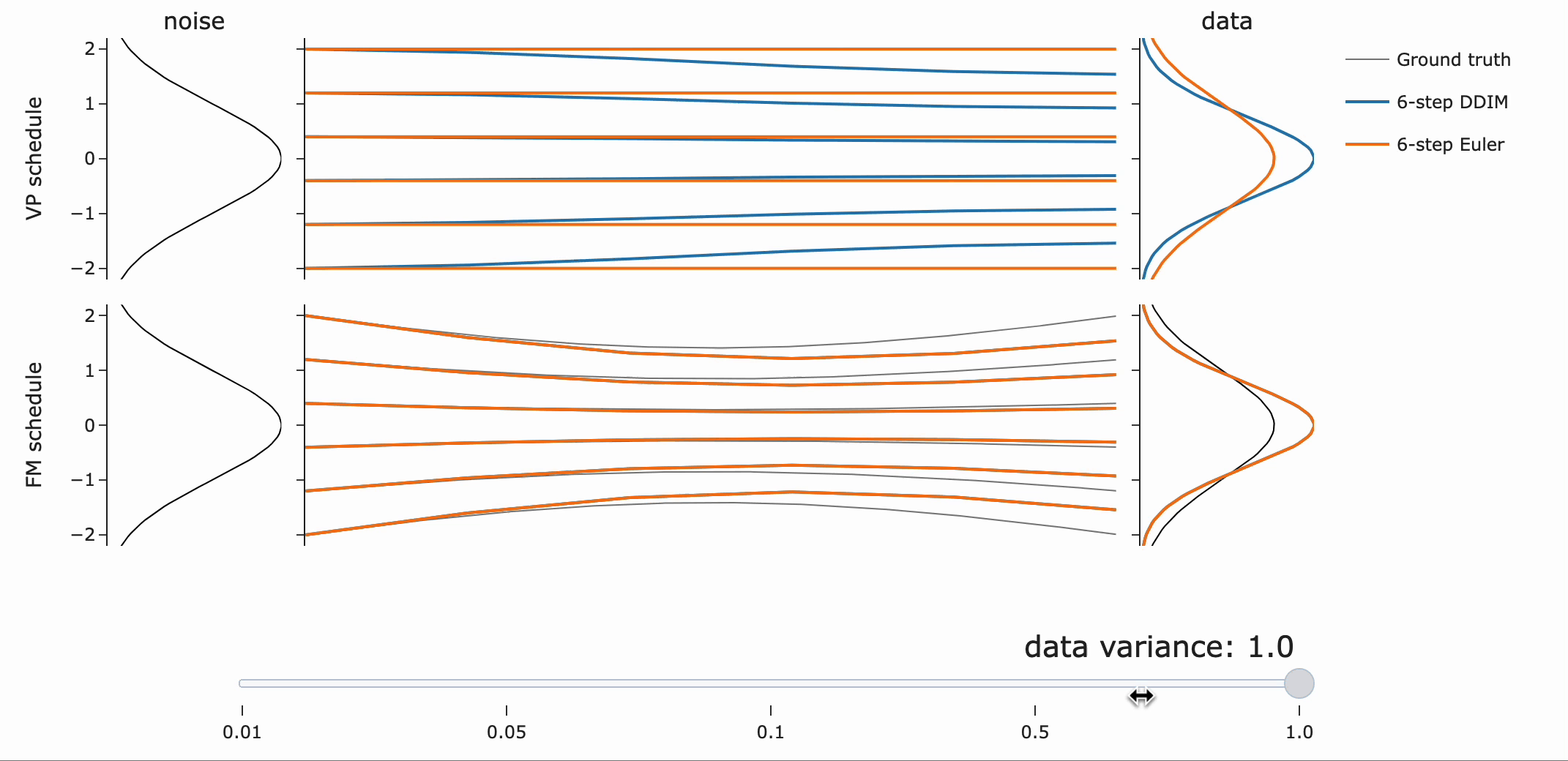
VP는 넓은 분포에 대해 더 나은 path (straighter)를 제공하는 반면, Flow matching은 좁은 분포에서 잘 동작한다는 점에 주목하라고 합니다.(?)

자… 정리해봅시다.

1. Sampler도 동일 : DDIM과 flow matching의 sampler는 동일하며, noise scheduling에 linear scaling을 해도 “invariant” 합니다.
2. Straightness misnomer : Flow matching이 single point를 예측할 때 직선이며, 실제 분포에서는 다른 sampler가 더 straight 할 수 있습니다.
3. 최적의 integration method는 결국 data distribution에 따라!

4. Training

Diffusion model은 \(\hat{\bf x} = \hat{\bf x}({\bf z}_t; t)\)를 예측하거나, \(\hat{\boldsymbol \epsilon} = \hat{\boldsymbol \epsilon}({\bf z}_t; t)\)를 예측하도록 학습합니다.

\[\mathcal{L}(\mathbf{x}) = \mathbb{E}_{t \sim \mathcal{U}(0,1), \boldsymbol{\epsilon} \sim \mathcal{N}(0, \mathbf{I})} \left[ \textcolor{green}{w(\lambda_t)} \cdot \frac{\mathrm{d}\lambda}{\mathrm{d}t} \cdot \lVert\hat{\boldsymbol \epsilon} - {\boldsymbol \epsilon}\rVert_2^2 \right],\]

여기서 \(\lambda_t = \log(\alpha_t^2 / \sigma_t^2)\) log SNR이며, \(\textcolor{green}{w(\lambda_t)}\)는 loss의 균형을 맞춰주는 weighting function입니다. 이때 \(\mathrm{d}\lambda / {\mathrm{d}t}\)는 종종 weighting function에 합쳐지기도 하지만, design choic를 명확하게 하는데 도움이 되므로 disentangle 했습니다.

Flow matching또한 위 objective function과 딱 맞아떨어집니다.

\[\mathcal{L}_{\mathrm{CFM}}(\mathbf{x}) = \mathbb{E}_{t \sim \mathcal{U}(0,1), \boldsymbol{\epsilon} \sim \mathcal{N}(0, \mathbf{I})} \left[ \lVert \hat{\bf u} - {\bf u} \rVert_2^2 \right]\]

여기서 \(\hat{\bf u}\)의 정의를 생각해보면 \({\boldsymbol \epsilon}\)의 MSE로도 표현할 수 있습니다.

How do we choose what the network should output?

아래 표는 다양한 네트워크 출력을 요약한 것입니다. Training objective 관점에서 보면, 모두 \(\epsilon\)-MSE앞에 추가적인 가중치를 가지는 것이며, weighting function으로 표현할 수 있습니다.

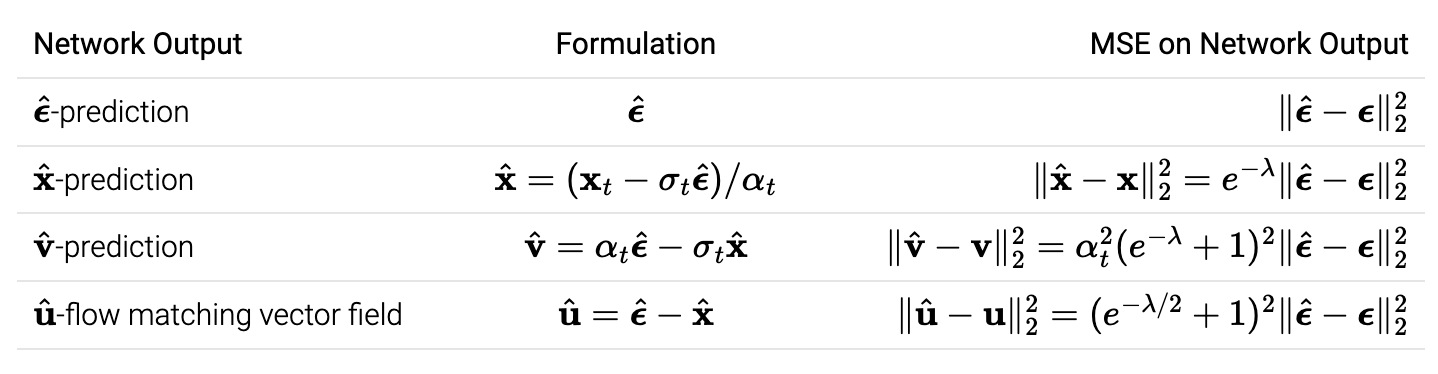
실제 학습에서는 모델 출력이 중요한 차이를 만들 수 있다고 합니다. 예를 들어,

• \(\hat{\boldsymbol \epsilon}\)-prediction은 높은 노이즈 수준에서 문제가 될 수 있습니다. \(\alpha_t\)가 0으로 감에 따라, \(\hat{\bf x} = ({\bf x}_t - \sigma_t \hat{\boldsymbol \epsilon}) / \alpha_t\)에서 작은 변화가 큰 loss로 나타날 수 있기 때문.
• 비슷한 이유로 \(\hat{\bf x}\)는 낮은 노이즈 수준에서 문제가 될 수 있습니다.

따라서 \(\hat{\bf v}\)과 flow matching vector field \(\hat{\bf u}\)에 적용되는, \(\hat{\bf x}\), \(\hat{\bf \epsilon}\)의 조합을 선택하는 것은 heuristic 하다고 합니다.

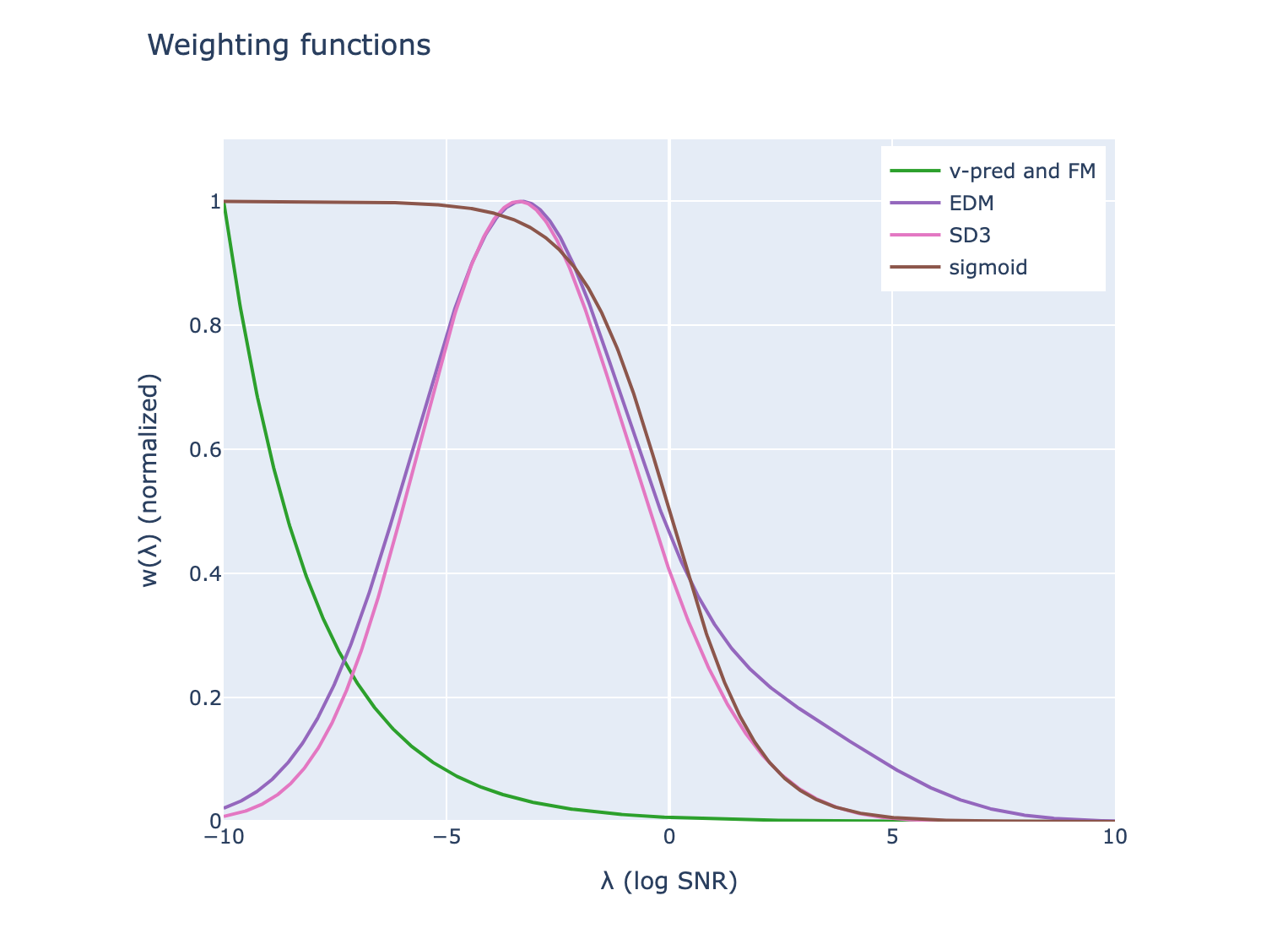
How do we choose the weighting function?

weighting function는 손실에서 가장 중요한 부분입니다. Loss 관점에서 다음의 결론에 도달합니다.

Flow matching weighting == diffusion weighting of vv-MSE loss + cosine noise schedule.

자주 사용되는 weight function의 \(\lambda\)를 나타내면 다음과 같습니다.

How do we choose the training noise schedule?

사실 noise scheduling은 학습에서 가장 중요도가 낮고, 간단하게만 주의하면 된다고 합니다.

1. Training loss는 noise schedule에 “invariant”합니다. [Noise schedules considered harmful]

\(\mathcal{L}(\mathbf{x}) = \int_{\lambda_{\min}}^{\lambda_{\max}} w(\lambda) \mathbb{E}_{\boldsymbol{\epsilon} \sim \mathcal{N}(0, \mathbf{I})} \left[ \|\hat{\boldsymbol{\epsilon}} - \boldsymbol{\epsilon}\|_2^2 \right] \, d\lambda\) 이므로, \(\lambda_{\max}, \lambda_{\min}\)에만 관련이 있는데, 실제로는 clean data, pure noise를 선택해야하므로…

1. Sampling noise scheduling과 비슷하게 training시에도 linear scaling에 “invariant”합니다. 노이즈 스케줄의 핵심 특성은 log SNR (\(\lambda_t\)​)

2. 학습과 샘플링에 대해 완전히 다른 noise scheduling을 선택할 수 있습니다.

   • Training: Monte Carlo 추정치의 분산을 최소화하는 노이즈 스케줄이 바람직합니다.
   • Sampling: ODE/SDE 샘플링 궤적의 이산화 오류 및 모델 곡률과 더 관련이 있습니다.

자.. 정리해봅시다.

1. Equivalence in weightings : Flow matching에서 사용되는 weight function은 우연히도 Diffusion에서 자주 사용되는 weight function과 일치합니다.

2. Difference in network outputs : Flow matching에서 제안된 새로운 네트워크 output은 \(\hat{\bf x}\), \(\hat{\bf \epsilon}\)의 균형을 적절히 맞추며, \(\hat{\bf v}\)와 유사합니다.

3. Insignificance of training noise schedule : Noise schedule은 training objective에 중요하지는 않지만 효율성에 영향을 미칠 수 있습니다.

Diving deeper into samplers

Reflow operator

Flow matching의 reflow 연산은 noise와 data point를 직선으로 연결합니다. 이는 deterministic sampler를 이용해 얻을 수 있는데, noise를 기반으로 모델은 이를 직접 예측하도록 학습할 수 있습니다. (diffusion에서는 이 접근법이 첫 번째 distillation 기법 중 하나로 사용되었다고 합니다)

Deterministic sampler vs. stochastic sampler

지금까지 deterministic sampler에 대해서만 논의했으나… DDPM 같은 stochastic한 sampler를 이용할 수 있습니다.

DDPM sampling step을 \(\lambda_t\)에서 \(\lambda_t + \Delta \lambda_t\)로 이동시키는 것은, \(\lambda_t + 2 \Delta \lambda_t\)까지 DDIM으로 이동시킨 다음, forward process로 noise를 추가하는 것과 \(\lambda_t + \Delta \lambda_t\) 동일합니다.

개별 샘플 관점에서는 꽤 달라보이지만, 모든 샘플 관점에서는 동일한 분포를 갖습니다. DDIM에서 renoising 하는 비율을 조절할 수 있는데, 이를 “churn” 이라 하며, 초기 샘플에서 모델 예측의 가중치를 줄이고, 후반 샘플에서 가중치를 증가시키는 효과를 가져옵니다.

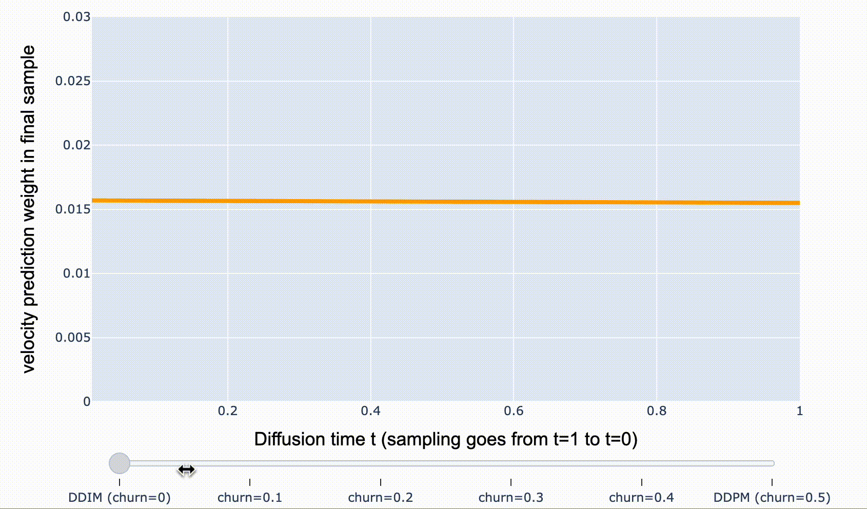
• DDIM( \(\text{churn}=0\)): \({\mathbf{v}}_t\)​-prediction weight가 시간에 따라 균일
• DDPM: 샘플링 후반부에 \(\hat{\mathbf{v}}_t\)-prediction weight가 더 집중

최종 샘플링은 샘플링 중 만들어진 \(\hat{\mathbf{v}}_t\)과 noise \(\epsilon\)으로 표현

\[{\bf z}_0 = \sum_t h_t \hat{\bf v}_t + \sum_t c_t {\bf e}\]

SDE and ODE Perspective

수식이 너무 많아서 결론만 전달하자면

‘Diffusion, flow matching 두 framework가 fundamentally 동일함을 수식으로도 보일 수 있다.’

(수식은 건너뛰어도 됩니다.)

Diffusion models

Forward process는 다음의 SDE로 표현할 수 있습니다.

\[\mathrm{d} {\bf z}_t = f_t {\bf z}_t \mathrm{d} t + g_t \mathrm{d} {\bf z} ,\]

생성과정(Reverse process)은 다음과 같습니다. \(\mathrm{d} {\bf z}_t = \left( f_t {\bf z}_t - \frac{1+ \eta_t^2}{2}g_t^2 \nabla \log p_t({\bf z_t}) \right) \mathrm{d} t + \eta_t g_t \mathrm{d} {\bf z} ,\)

이때 \(\nabla \log p_t({\bf z_t})\)를 forward process의 score 라 합니다.

DDIM : \(\eta_t = 0\) DDPM : \(\eta_t = 1\)

Flow matching

ODE로 표현하면 다음과 같습니다.

\[\mathrm{d}{\bf z}_t = {\bf u}_t \mathrm{d}t.\]

만약 \({\bf z}_t = \alpha_t {\bf x} + \sigma_t {\boldsymbol \epsilon}\)을 가정하면,

\[{\bf u}_t = \dot{\alpha}_t {\bf x} + \dot{\sigma}_t {\boldsymbol \epsilon}\]

생성과정은 ODE를 시간에 따라 역전시키고, \(u_t\)를 \(z_t\)에 대한 conditional expectation로 대체한 값입니다.

\[\mathrm{d} {\bf z}_t = ({\bf u}_t - \frac{1}{2} \varepsilon_t^2 \nabla \log p_t({\bf z_t})) \mathrm{d} t + \varepsilon_t \mathrm{d} {\bf z}\]

Equivalence of the two frameworks

• From diffusion to flow matching: \(\alpha_t = \exp\left(\int_0^t f_s \mathrm{d}s\right) , \quad \sigma_t = \left(\int_0^t g_s^2 \exp\left(-2\int_0^s f_u \mathrm{d}u\right) \mathrm{d} s\right)^{1/2} , \quad \varepsilon_t = \eta_t g_t .\)
• From flow matching to diffusion: \(f_t = \partial_t \log(\alpha_t) , \quad g_t^2 = 2 \alpha_t \sigma_t \partial_t (\sigma_t / \alpha_t) , \quad \eta_t = \varepsilon_t / (2 \alpha_t \sigma_t \partial_t (\sigma_t / \alpha_t))^{1/2} .\)

Closing takeaways

이 포스팅을 통해 다음을 기억합시다!

• Network output:
  Flow matching은 network output으로 (기존 diffusion model 사용되는 것과 다른) vector field parametrization를 제안. Output은 higher-order samplers를 사용할 때 차이가 발생하며, training dynamics에도 영향

• Sampling noise schedule:
  Flow matching은 \(\alpha_t = 1-t\) \(\sigma_t = t\) sampling noise schedule 활용하며, 이는 DDIM과 동일.