[Paper Reivew] Flow Matching Gudie and Code-(2. Quick tour)
Flow matching의 comprehensive, self-contained review 입니다.

NeurIPS 2024 Tutorial (?) [Paper] [github]
Yaron Lipman, Marton Havasi, Peter Holderrieth, Neta Shaul, Matt Le, Brian Karrer, Ricky T. Q. Chen, David Lopez-Paz, Heli Ben-Hamu, Itai Gat
FAIR at Meta | MIT CSAIL | Weizmann Institute of Science
9 Dec 2024
리키 첸이 설명하는 Flow matching… 83페이지나 되네요.
TL;DR
- Flow Matching(FM)은 velocity field를 학습해 소스 분포 \(p\)를 타겟 분포 \(q\) 로 변환하는 확률 경로 \(p_t\)를 만드는 framework.
- FM은 다양한 상태 공간(이산, 리만 다양체)과 마르코프 과정(CTMC, CTMP)으로 확장 가능하며, Diffusion Models 등 기존 모델들을 통합적으로 이해할 수 있는 틀을 제공.
전체 포스팅
1. Introduction
Flow matching이란 velocity field 학습을 위한 framework입니다. 각 velocity field는 ODE를 풂으로써, flow \(\psi_t\)를 정의합니다.
Flow matching의 목표는 source sample \(X_0 \sim p\)에서 target sample \(X_1 := \psi_1(X_0)\) 로 가는 flow를 만드는 것입니다. (제일 왼쪽 그림)
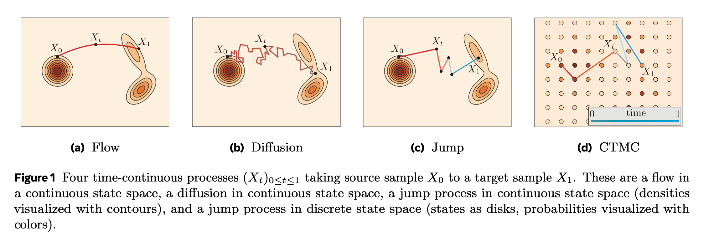
뒤에서는 위 과정(Flow, diffusion, jump, CTMC in discrete space)들을 포함한 어떠한 modality던, 어떤 general CTMP이던, Generator Matching으로 통합하는 과정을 설명합니다.
CTMC = Continuous Time Markov Chains
CTMP = Continuous Time Markov Processes
이렇게 GM으로 확장해도 결국 2가지 step으로 구성된다는 것을 명심해야 합니다.
- Source \(p\)와 target \(q\)를 잇는 probability path \(p_t\) 고르기
- Generator를 학습시켜, \(p_t\)를 implement하는 CTMP를 정의
예를 들어 FM에서는 velocity field를 학습하여, \(p_t\)를 implement하는 \(\psi_t\) 를 정의합니다.
Diffusion model과의 관계
사실 CTMP 과정을 simulation-free training 방법으로 접근한 것은 Diffusion model이 먼저라고 합니다.
Flow matching 관점에서 Diffusion model은
- 특정 SDE로부터 모델링 된 “forward noising process“로 source와 target을 interpolate하는 probability path \(p_t\)를 구성합니다. 이 SDE 들은 closed form marginal probabilities를 가지며, score function을 통해 diffusion process의 generator를 parameterize 합니다.
- 이런 parameterization는 forward process를 거꾸로 하는 방식으로 진행되며 결과적으로 diffusion model은 marginal probabilities의 score function을 학습하게 됩니다.
기존의 score 함수 외에도 noise prediction, denoisers, v-prediction 같은 대안적 접근법이 제안되었는데, 우연히도 v-prediction은 특정 확률 경로 \(p_t\) 에 대한 velocity prediction과 일치합니다.
2. Quick tour and key concepts
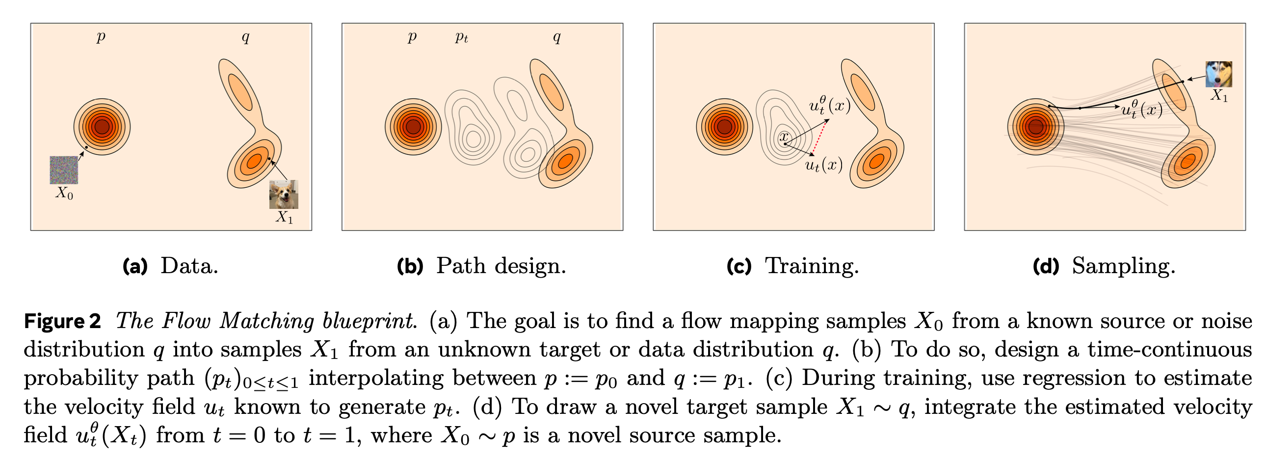
Flow matching의 goal: 주어진 target 분포 \(q\)로부터, 새로운 샘플을 만들 수 있는 모델을 구축하는 것.
간단하게 설명하자면 다음과 같습니다.
- probability path, \((p_t)_{0 \leq t \leq 1}\) :
- known source distribution \(p_0 = p\)로부터, target distribution \(p_1 = q\)로 이어지는 확률 경로.
- Velocity field, \(u_t\) :
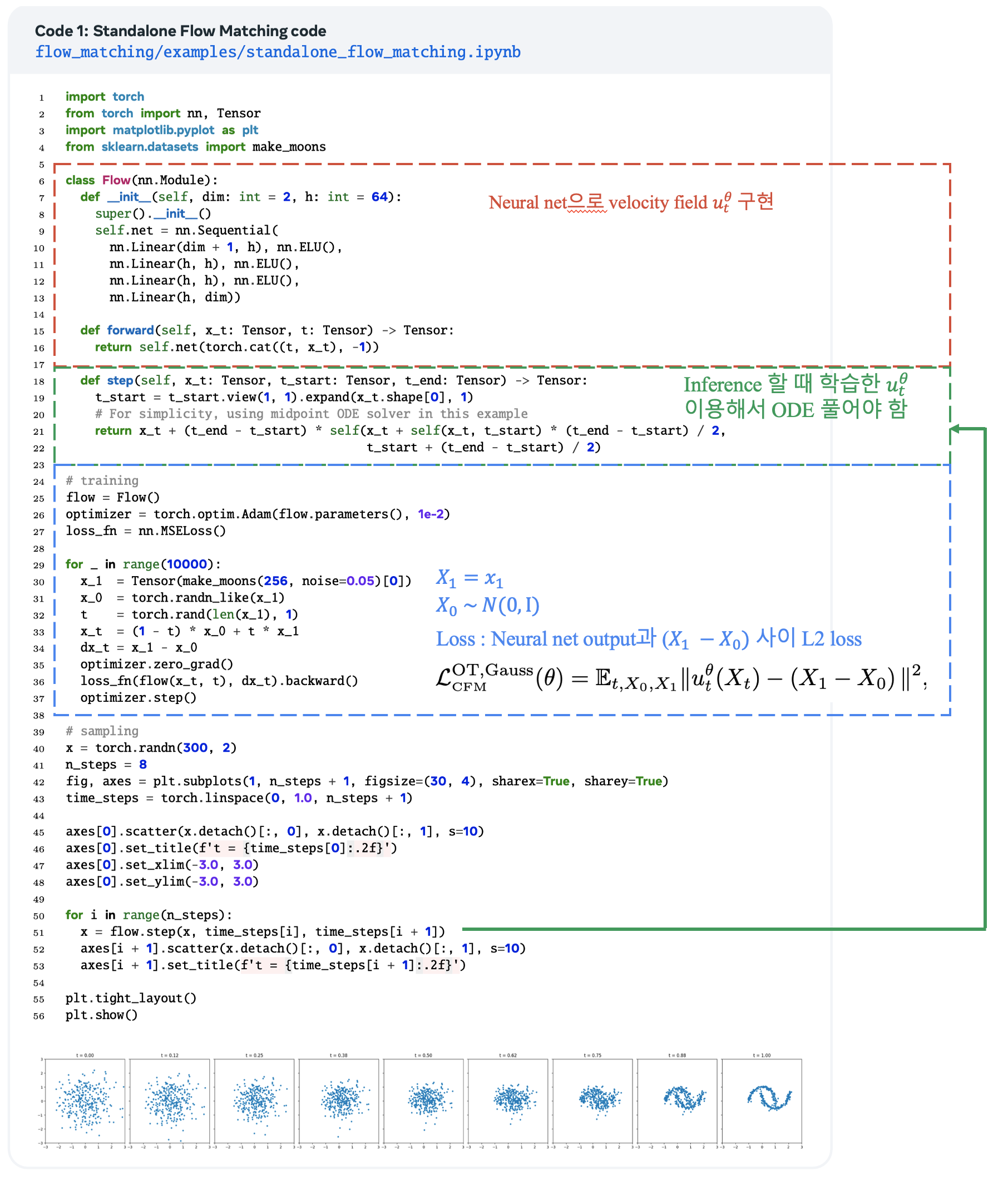
- Probability path \(p_t\)를 따라 샘플이 이동하는 순간적인 속도를 나타내는 Velocity field, \(u_t^\theta\) 를 신경망으로 학습.
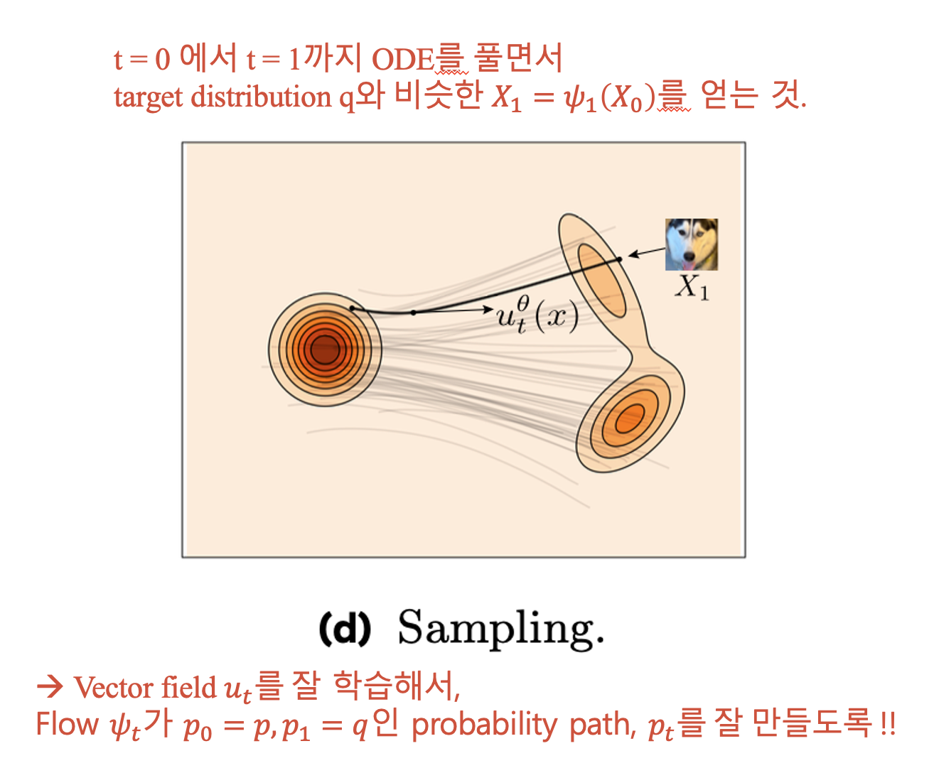
- 학습이 끝난 뒤, target 분포 \(X_1 \sim q\)에서 sampling 가능!
- Source 분포 \(X_0 \sim p\)에서 sampling 하고,
- \(u_t^\theta\) 로 정해지는 ODE 풀기.
자세하게 보자면… ODE는 time-dependent vector field \(u : [0, 1] \times \mathbb{R}^d \rightarrow \mathbb{R}^d\)에 의해 정의되며, flow matching에서는 neural network로 modeling 합니다.
Velocity field, \(u_t\) 는 다음과 같은 time-dependent flow를 결정합니다.
Flow \(\psi_t\)가 다음을 만족하면, \(u_t\) 는 probability path \(p_t\)를 generate 할 수 있습니다.
\[X_t := \psi_t(X_0) \sim p_t \text{ for } X_0 \sim p_0\]위 식에서 결국 \(u_t\) 만 있으면, ODE를 풂으로써, \(p_t\)로부터 sampling 할 수 있습니다.
정리하자면 다음과 같습니다.
\(u_t\) 를 잘 얻기 위해 2 step 으로 나눠서,
1) Design a probability path, \(p_t\)
2) Train a Velocity field, \(u_t^\theta\)
Design probability path, \(p_t\)
예를 들어 source 분포 \(p := p_0 = \mathcal{N}(x | 0, I)\)를 data example \(X_1 = x_1\)로 conditioning해서, probability path, \(p_t\) 를 구성할 수 있습니다.
\[p_t(x) = \int p_{t|1}(x|x_1) q(x_1) dx_1, \quad \text{where } p_{t|1}(x|x_1) = \mathcal{N}(x | t x_1, (1 - t)^2 I).\]이 path는 conditional optimal-transport or linear path라 불리는데, 뒤에서 다룰 이상적인 특징이 있다고 합니다. 이를 이용하면 Random variable \(X_t\)를 다음과 같이 정의할 수 있습니다.
\[X_t = t X_1 + (1 - t) X_0 \sim p_t.\]한 줄 요약.
\(X_0 \sim p\), \(X_1 \sim q\)의 linear combination으로 \(X_t \sim p_t\) 정의 가능.
Train Velocity field, \(u_t^\theta\)
Velocity field, \(u_t^\theta\) 를 이상적인 probability path, \(p_t\) 를 만드는 \(u_t\) 와 같아지도록 학습하는 것이 목표.
\[\mathcal{L}_{FM}(\theta) = \mathbb{E}_{t, X_t} \left[ \| u^\theta_t(X_t) - u_t(X_t) \|^2 \right], \quad t \sim \mathcal{U}[0,1], \, X_t \sim p_t.\]하지만.. probability path, \(p_t\) 는 두 개의 고차원 분포 사이의 joint transformation을 gorverning하므로 직접 구현은 어렵다고 합니다.
다행히도, single target example에 대해 conditioning만 해준다면 상당히 간단하게 이를 해결할 수 있다고 합니다. 따라서 \(X_t\)를 conditioning 해주면 다음과 같습니다.
\[X_{t|1} = t x_1 + (1 - t) X_0 \sim p_{t|1}(\cdot | x_1) = \mathcal{N}(\cdot | t x_1, (1 - t)^2 I).\]이를 이용해 conditional probability path, \(p_{t|1}(\cdot |x_1)\) 를 만드는 conditional velocity field를 구할 수 있습니다.
\[u_t(x | x_1) = \frac{x_1 - x}{1 - t}.\]따라서 conditional flow matching loss 는 다음과 같습니다.
\[\mathcal{L}_{\text{CFM}}(\theta) = \mathbb{E}_{t, X_t, X_1} \| u_t^\theta(X_t) - u_t(X_t | X_1) \|^2, \quad \text{where } t \sim \mathcal{U}[0, 1], X_0 \sim p, X_1 \sim q.\]뒤에서 살펴보겠지만, conditional loss와 일반 loss는 같은 gradient 값을 갖는다고 합니다.
\[\nabla_\theta \mathcal{L}_{\text{FM}}(\theta) = \nabla_\theta \mathcal{L}_{\text{CFM}}(\theta).\]따라서 최종적으로, \(u_t(x | x_1)\)를 \(\mathcal{L}_{\text{CFM}}(\theta)\)에 대입하면,
\[\mathcal{L}_{\text{CFM}}^{\text{OT,Gauss}}(\theta) = \mathbb{E}_{t, X_0, X_1} \| u_t^\theta(X_t) - (X_1 - X_0) \|^2\] \[\text{where } t \sim \mathcal{U}[0, 1], X_0 \sim \mathcal{N}(0, I), X_1 \sim q.\]한 줄 요약.
conditioning 해주고, 으쌰으쌰 계산하면 \(\mathcal{L}_{\text{CFM}}^{\text{OT,Gauss}}(\theta) = \mathbb{E}_{t, X_0, X_1} \| u_t^\theta(X_t) - (X_1 - X_0) \|^2\) 얻음.