[Paper Reivew] Flow Matching Gudie and Code-(3. Flow models)

전체 포스팅

• 1편, Quick tour
• 2편, Flow Models
• 3편, Flow Mathcing

3. Flow models

이번 섹션에서는 Flow에 대해 소개합니다. 먼저 간단한 형태의 Flow Matching에서 시작하여, (다음 section에서) Markov process로 일반화하는 과정을 거칩니다. 다음의 사실을 알고 가야합니다.

1. Flow는 CTMP의 가장 간단한 형태입니다. 임의의 source 분포에서, 임의의 target 분포로 transform할 수 있습니다.
2. ODE의 solution을 approximation 하는 것 대신에 flow는 sampling 될 수 있습니다.
3. Deterministic한 방식으로 unbiased model likelihood estimation이 가능합니다.

---

3.1. Random vectors

(생략)

3.2. Conditional densities and expectations

(생략)

3.3. Diffeomorphisms and push-forward maps

생략...하십쇼

\( C^r(\mathbb{R}^m, \mathbb{R}^n) \)을 \( r \)-차 미분 가능한 연속 함수 \( f : \mathbb{R}^m \rightarrow \mathbb{R}^n \)들의 집합이라 정의하면, Diffeomorphism (미분동형사상)이란 역함수도 \( r \)-차 미분 가능한 가역함수 들의 집합을 의미합니다.

\[ \psi \in C^r(\mathbb{R}^n, \mathbb{R}^n) \quad \text{with} \quad \psi^{-1} \in C^r(\mathbb{R}^n, \mathbb{R}^n). \]

자... Random Variable \( X \sim p_X \), \( Y = \psi(X), \quad \text{where} \quad \psi : \mathbb{R}^d \rightarrow \mathbb{R}^d \)이 \( C^1 \) diffeomorphism이라 가정합시다. \( Y \)의 PDF \( p_Y \)는 \( p_X \)의 "push-forward"라 부르며 다음과 같이 계산할 수 있습니다:

\[ p_Y(y) = p_X(\psi^{-1}(y)) \lvert \det \partial_y \psi^{-1}(y) \rvert. \]

Details

\[ \mathbb{E}[f(Y)] = \mathbb{E}[f(\psi(X))] = \int f(\psi(x)) p_X(x) \, dx = \int f(y) \underbrace{p_X(\psi^{-1}(y)) \lvert \det \partial_y \psi^{-1}(y) \rvert \,}_{p_Y} dy. \]

이때 \( \partial_y \psi(y) \)는 Jacobian matrix를 의미합니다:

\[ [\partial_y \phi(y)]_{i,j} = \frac{\partial \phi^i}{\partial x^j}, \quad i, j \in [d]. \]

또한 push-forward operator를 \( \sharp \) 으로 정의합니다:

\[ [\psi_\sharp p_X](y) := p_X(\psi^{-1}(y)) \lvert \det \partial_y \psi^{-1}(y) \rvert. \]

3.4. Flows as generative models

반복하지만 Generative model의 목표는

• Source 분포 \(p\)로 부터의 sample \(X_0 = x_0\) \(\to\) Target 분포 \(q\)의 sample \(X_1 = x_1\)으로 transform 하는 것!

---

Flow model은 continuous-time Markov process \((X_t)_{0\leq t \leq 1}\) 이며, RV \(X_0\)에 flow \(\psi_t\)를 적용해, 최종적으로 \(t = 1\)일 때 Target distribution으로 가도록 합니다.

\[X_t = \psi_t(X_0), \quad X_0 \sim p, \,\text {s.t.} \quad X_1 = \psi_1(X_0)\sim q\]

Markov Proof

\( C^r \) flow란 시간 \( t \)에 따라 입력 \( x \)를 변환하는 mapping \( \psi_t: [0, 1] \times \mathbb{R}^d \to \mathbb{R}^d \)인데, \( \psi_t \)가 \( t \in [0, 1] \) 안에서 \( C^r \)-diffeomorphism인 것을 말합니다. 임의의 \( 0 \leq t < s \leq 1 \)에 대해서 다음을 만족합니다:

\[ X_s = \psi_s(\psi_t^{-1}(\psi_t(X_0))) = \psi_{s|t}(X_t) \]

즉, \( X_t \) 이후의 state는 \( X_t \)에만 의존함을 의미하므로, Markov 입니다.

3.4.1 Equivalence between flows and velocity fields

결론만 전달하자면 \(C^r\) flow와 \(C^r\) velocity field \(u_t\)는 동일합니다.

직관적으로 이해하자면

• Flow: 시간에 따라 상태를 변환하는 전체 궤적.
• velocity field: 특정 시간에서의 순간적인 변화율.

Flow로부터 velocity field를 얻으려면 시간 변화율 계산해야 하고, Velocity field로부터 flow 얻으려면 ODE를 풀어야합니다.

\[u_t(x) = \dot{\psi}_t\left(\psi_t^{-1}(x)\right),\]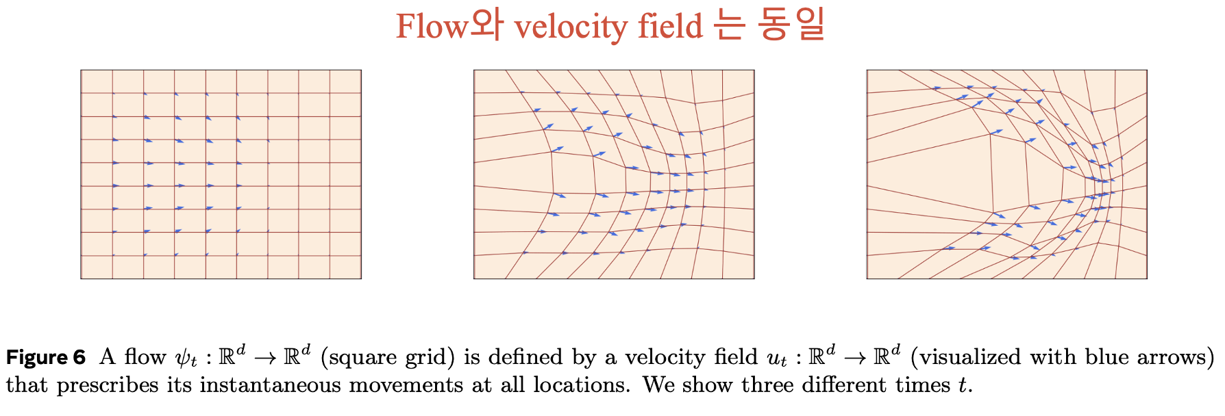

3.4.2. Computing target samples from source samples

Target sample \(X_1\) (일반화하자면 \(X_t\))를 계산하기 위해서는 \(X_0 = x_0\)에서 시작해, \(u_t^\theta\)를 가지고, ODE를 Numerically 풀면 됩니다.
그 중 하나의 예시가 Euler Method.

Euler method

간단한 방법 중 하나는 Euler method입니다. (참고: Code 1에서는 second-order midpoint method 사용)

\[ X_{t+h} = X_t + h u_t(X_t), \]

Euler Method는 \( X_t \)의 first-order Taylor expansion과 동일한데:

\[ X_{t+h} = X_t + h \dot{X}_t + o(h) = X_t + h u_t(X_t) + o(h), \]

여기서, \( o(h) \)는 \( o(h)/h \to 0 \)인 함수들을 의미합니다.

• Euler Method는 각 시간 스텝 \( h \)에서 \( o(h) \) 크기의 오류를 포함합니다.
• \( n = 1/h \) 스텝 동안 총 누적 오류는 \( o(1) \)이 되며, \( h \to 0 \)으로 스텝 크기를 줄이면 이 오류는 사라집니다.

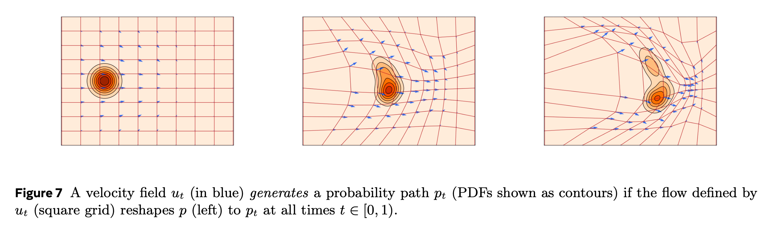
3.5. Probability paths and the Continuity Equation

Time-dependent probability \((p_t)_{0 \leq t \leq 1}\)을 probability path라 합니다. 지금 상황에서 중요한 probability path는 flow model \(X_t = \psi_t(X_0)\)의 marginal \(\text{PDF}\) 이며, push-forward 공식을 통해 표현할 수 있습니다.

\[p_t(x) = [\psi_{t\sharp} p](x).\]

임의의 probability path, \(p_t\)로 부터, 다음을 정의합니다.

\[u_t \color{blue}{\textbf{ generates }} \color{black}p_t \text{ if } X_t = \psi_t(X_0) \sim p_t \text{ for all } t \in [0, 1).\]

이 방식으로, 우리는 velocity field, 그것들의 (equivalent) flow, generated probability path의 관게를 정립할 수 있습니다.

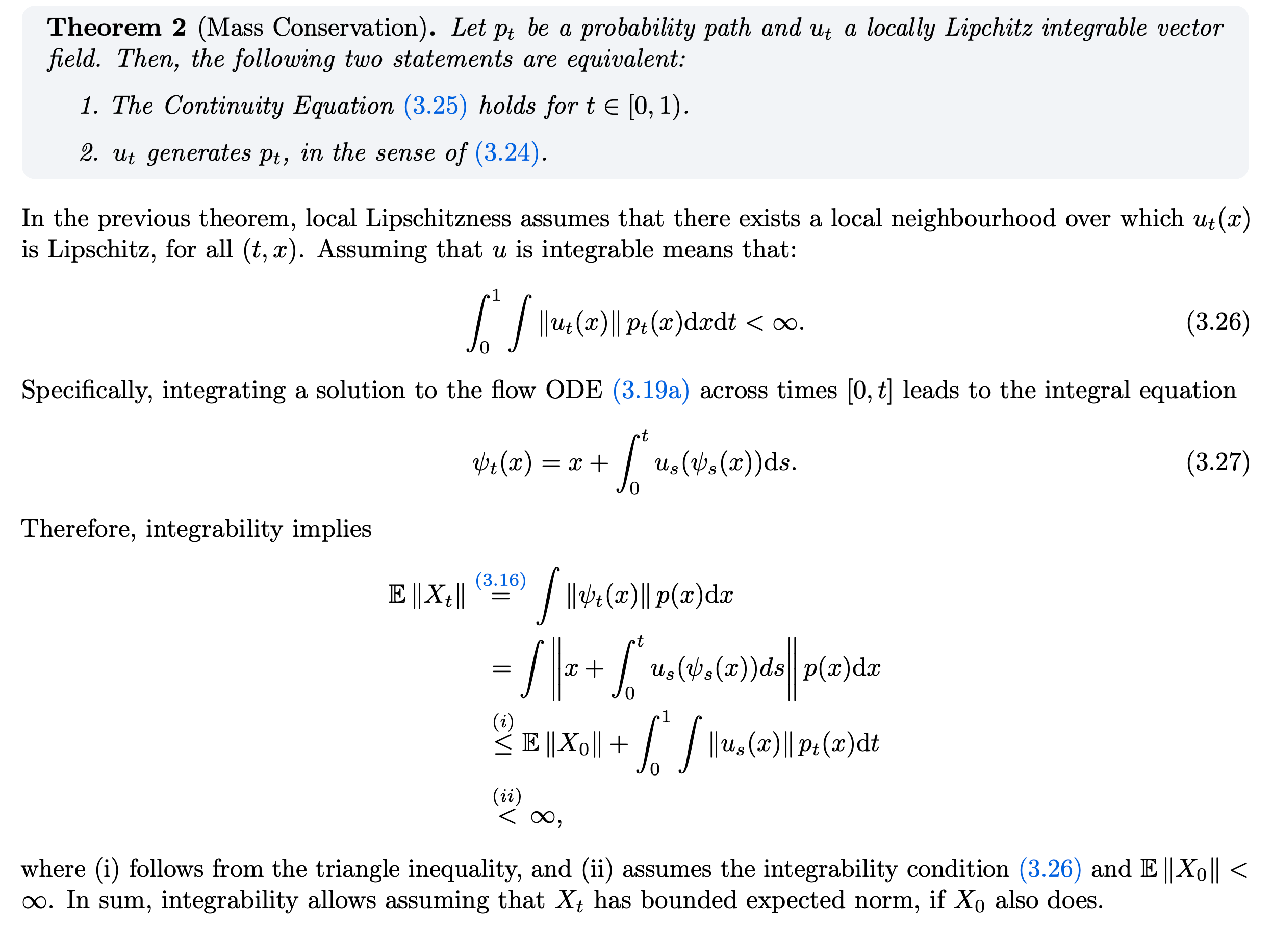
또한 다음 두 문장은 equivalent합니다.

1. \(\color{black} \text{Continuity Equation } \frac{d}{dt} p_t(x) + \operatorname{div}(p_t u_t)(x) = 0 \text{ holds for all } t \in [0, 1)\).
2. \(\color{black} u_t \color{blue}{\textbf{ generates }} \color{black}p_t \text{ if } X_t = \psi_t(X_0) \sim p_t \text{ for all } t \in [0, 1)\).

Proof

\( u_t \)가 \( p_t \)를 generate하는 것을 보이려면 \( (u_t, p_t) \)가 Continuity Equation을 만족함을 보이면 됩니다.

\[ \frac{d}{dt} p_t(x) + \operatorname{div}(p_t u_t)(x) = 0. \]

Divergence Theorem

Smooth vector field \( u : \mathbb{R}^d \to \mathbb{R}^d \)에 대해, 영역 \( D \) 내부에서의 divergence를 적분한 값은 영역 경계 \( \partial D \)를 빠져나가는 flux와 같습니다.

\[ \int_D \operatorname{div}(u)(x) \, dx = \int_{\partial D} \langle u(y), n(y) \rangle \, d s_y. \]

Divergence theorem을 이용해 integral-form으로 바꾸면 몇 가지 insights를 얻을 수 있습니다:

\[ \frac{d}{dt} \int_D p_t(x) \, dx = - \int_D \operatorname{div}(p_t u_t)(x) \, dx = - \int_{\partial D} \langle p_t(y) u_t(y), n(y) \rangle \, d s_y. \]

이를 해석하자면:

• 좌변은 영역 \( D \) 내부의 확률 질량의 변화율(시간적 변화)을 나타냅니다.
• 우변은 domain을 빠져나가는 probability flux를 나타냅니다.
• probability flux \( j_t(y) = p_t(y) u_t(y) \)는 확률 밀도 \( p_t(y) \)와 velocity field \( u_t(y) \)의 곱으로 정의되며, 이는 "확률 질량이 이동하는 방향과 크기"를 나타냅니다.

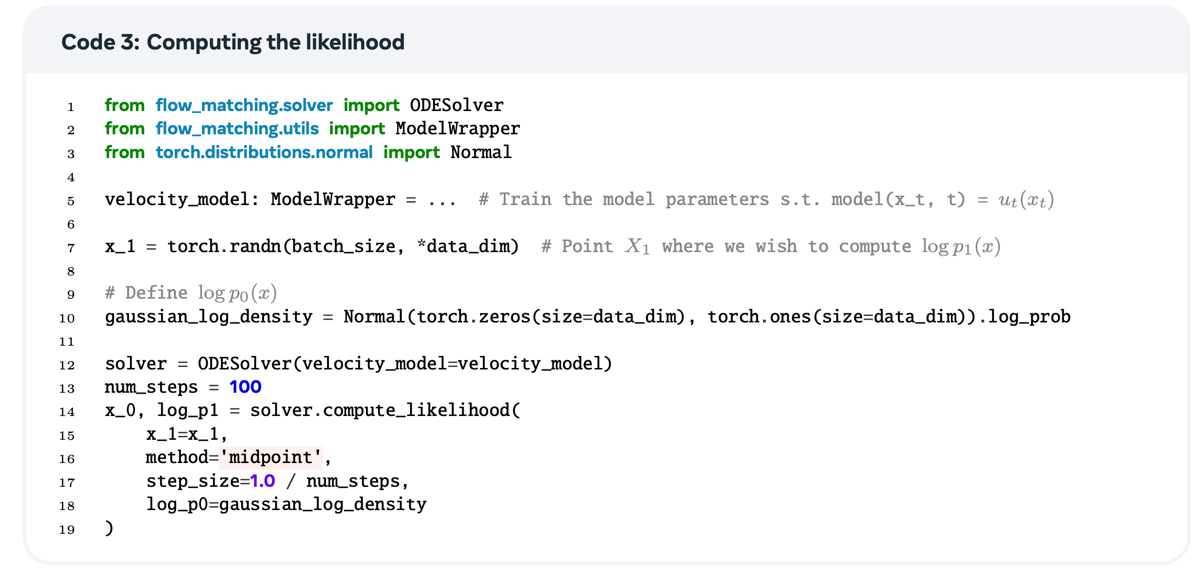
3.6. Instantaneous Change of Variables

Flow model을 사용하는 주요 장점 중 하나는 exact likelihood를 계산할 수 있다는 것입니다. 이는 Instantaneous Change of Variables라 불리는 Continuity Equation의 결과 덕분이라고 합니다.

\[\frac{d}{dt} \log p_t(\psi_t(x)) = -\text{div}(u_t)(\psi_t(x)),\]

위 식은 Flow ODE에 의해 정의되는 \(\psi_t(x)\)를 따라 샘플링하는 log-likelihood를 governing하는 ODE입니다. 하지만 이를 위해서는 ODE를 backward in time으로 simulation하는 과정이 필요합니다.

Log-Likelihood Estimation

Hutchinson's Trace Estimator를 사용해 근사하여, unbiased log-likelihood estimator를 얻습니다.

\[ \log p_1(\psi_1(x)) = \log p_0(\psi_0(x)) - \mathbb{E}_Z \int_0^1 Z^T \partial_x u_t(\psi_t(x)) Z \, dt. \]

\(\text{div}(u_t)(\psi_t(x))\) 계산과 다르게, 위 식을 계산하려면 vector-Jacobian product (JVP)를 통한 single backward pass를 이용해 계산할 수 있다고 합니다.

따라서 정리하자면, log-likelihood를 계산하기 위해 \( t =1 \to 0 \)로 ODE를 simulation하면 됩니다:

\[ \frac{d}{dt} \begin{bmatrix} f(t) \\ g(t) \end{bmatrix} = \begin{bmatrix} u_t(f(t)) \\ -\text{tr}[Z^T \partial_x u_t(f(t)) Z] \end{bmatrix}. \]

최종적으로 다음을 얻습니다:

\[ \log p_1(x) = \log p_0(f(0)) - g(0). \]

3.7. Training flow models with simulation

위 결과식을 이용해서, training data의 log-likelihood를 최대화하도록 flow model을 학습할 수 있습니다.

\[p_1^\theta \approx q\]

가 되도록 \(u_t^\theta\)를 학습하고자 하는데, 이는 KL-divergence등을 이용해 구현할 수 있습니다.

\[\mathcal{L}(\theta) = D_{\text{KL}}(q, p_1^\theta) = -\mathbb{E}_{Y \sim q} \log p_1^\theta(Y) + \text{constant}.\]

하지만 이 손실 함수와 그 gradient를 계산하려면, 훈련 과정에서 정확한 ODE 시뮬레이션이 필요합니다.

이와는 다르게, Flow matching은 simulation-free framework를 제공한다고 합니다.

---

Summary

정리하자면…

• Flow model은 CTMP \(X_t\) 이며, \(\text{RV } X_0\)에 flow \(\psi_t\)를 적용해, 최종적으로 \(t = 1\)일 때 Target distribution으로 가도록.

\[X_t = \psi_t(X_0), \quad X_0 \sim p, \,\text {s.t.} \quad X_1 = \psi_1(X_0)\sim q\]

• Velocity field \(u_t\)는 flow의 순간 변화율, ODE를 통해 flow와 상호 변환이 가능.
• Log-likelihood를 정확히 계산할 수 있지만, simulation이 필요.
• Source sample에서 target sample을 계산하려면 ODE 를 Numerically 풀어야 함!

전체 포스팅

• 1편, Quick tour
• 2편, Flow Models
• 3편, Flow Mathcing