[Paper Reivew] Flow Matching Gudie and Code-(4. Flow Matching)
Flow matching의 comprehensive and self-contained reviewd 입니다.

전체 포스팅
4. Flow Matching
Flow Matching (FM)은 “Flow Matching Problem” 이라는 문제를 풀기위한, flow model, \(u_t^\theta\)를 학습하기 위한 scalable 방법론입니다.
Flow Matching Problem : \(\text{Find } u_t^\theta \text{ generating } p_t, \quad \text{with } p_0 = p \text{ and } p_1 = q.\)
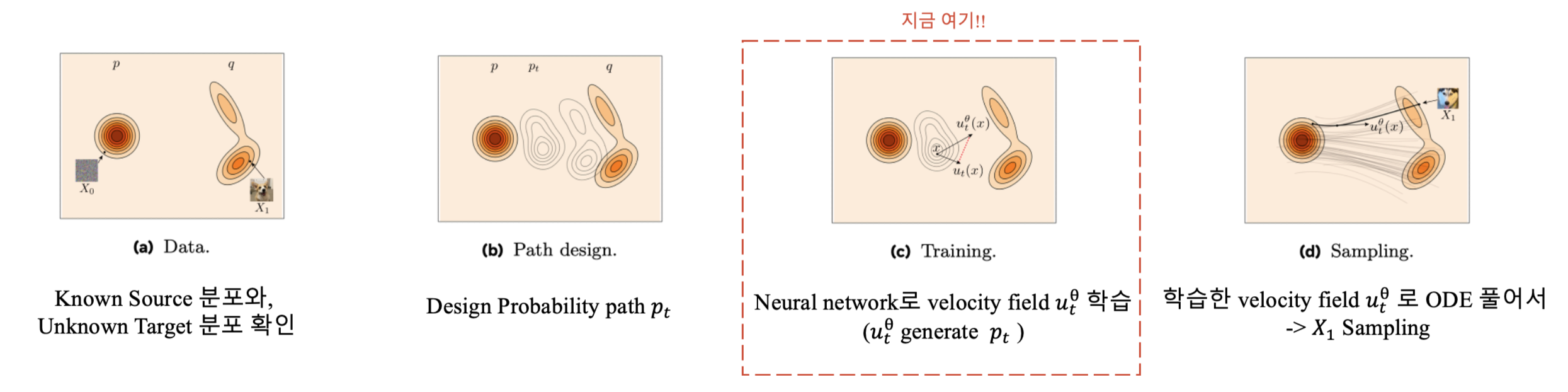
다시 아래 그림을 살펴봅시다.
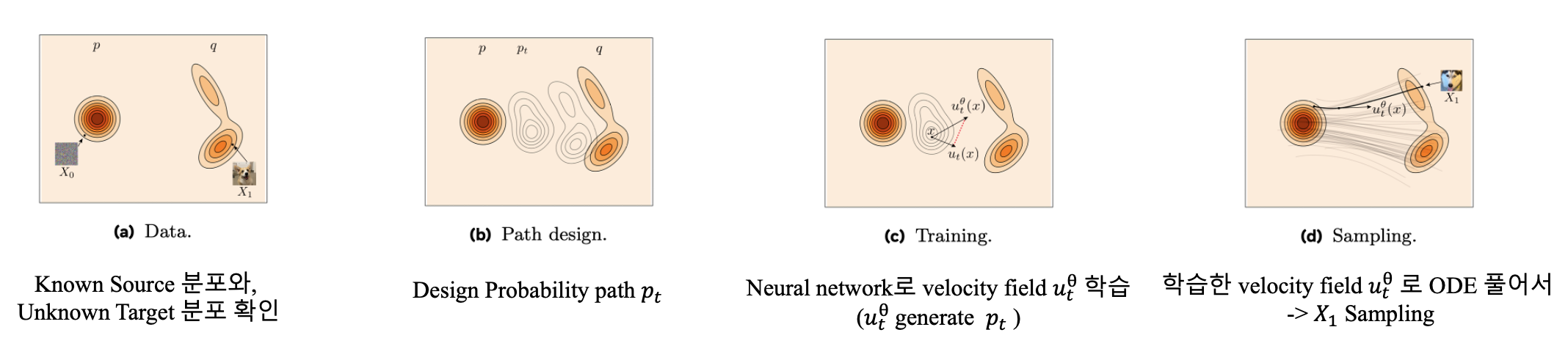
이 포스팅의 전체 흐름을 정리해보자면…
- Data 분포를 살펴봅니다.
- probability path, \(p_t\) 를 구하는 과정을 살펴봅니다.
- Generating velocity fields \(u_t(x)\)를 유도합니다.
- Conditioning을 일반화해도 \(u_t(x)\)가 \(p_t\) 를 generate 하는지 보입니다.
- Flow Matching loss를 정의합니다.
- 1~5에서 정리한 내용을 기반으로 Flow를 정의하고 이를 이용해 task를 간단화합니다. (FM의 핵심)
- (Case study) Linear conditional flow
- (Case study) Affine conditional flows
- Data coupling
- Guidance
4.1. Data
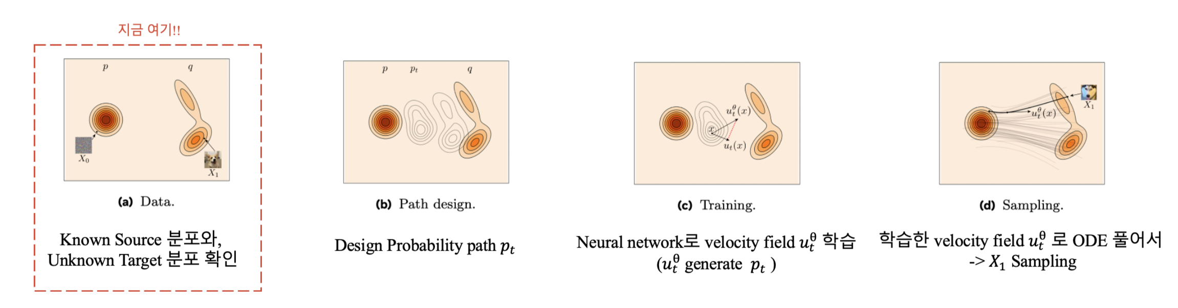
- Source sample : \(\text{RV } X_0 ~ p\), known distribution (e.g. Gaussian)
- Traget sample : \(\text{RV } X_1 ~ q\), Finite 크기의 dataset으로 주어짐.
Source 와 target은 independent or dependent 일 수 있으며, coupling 이라는 joint distribution을 형성합니다.
Independent : \((X_0, X_1) \sim \pi_{0,1}(X_0, X_1) = p(X_0)q(X_1)\) e.g. Gaussian noise에서 이미지 generate.
Dependent : \((X_0, X_1) \sim \pi_{0,1}(X_0, X_1),\) e.g.
- 저해상도 \(X_0\)에서 고해상도 \(X_1\) generate
- Masked image \(X_0\)에서 inpaint \(X_1\)
4.2. Building probability paths
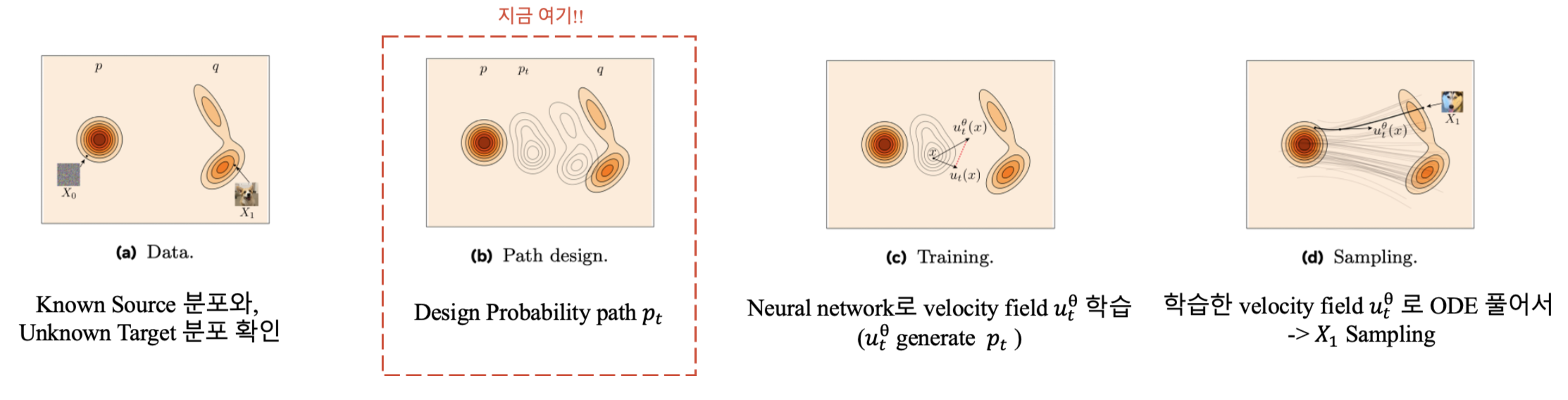
한 줄 요약. Conditional 전략을 취해, probability path \(p_t\) design을 간단히!
예를 들면, single target example \(X_1 = x_1\)로 conditioning 하는 경우 \(p_{t|1}(x|x_1)\) 를 얻을 수 있으며, 이를 marginalize하여 \(p_t\)를 구성할 수 있습니다.
\[p_t(x) = \int p_{t|1}(x|x_1) q(x_1) dx_1.\]이때 Boundary condition (B.C.)은 다음과 같습니다.
\[p_0 = p, \quad p_1 = q\]이 B.C. 은 conditional probability paths \(p_{t|1}(x|x_1)\)를 통해 다음과 같이 만족될 수 있다고 합니다.
\[p_{0|1}(x|x_1) = \pi_{0|1}(x|x_1), \quad p_{1|1}(x|x_1) = \delta_{x_1}(x),\]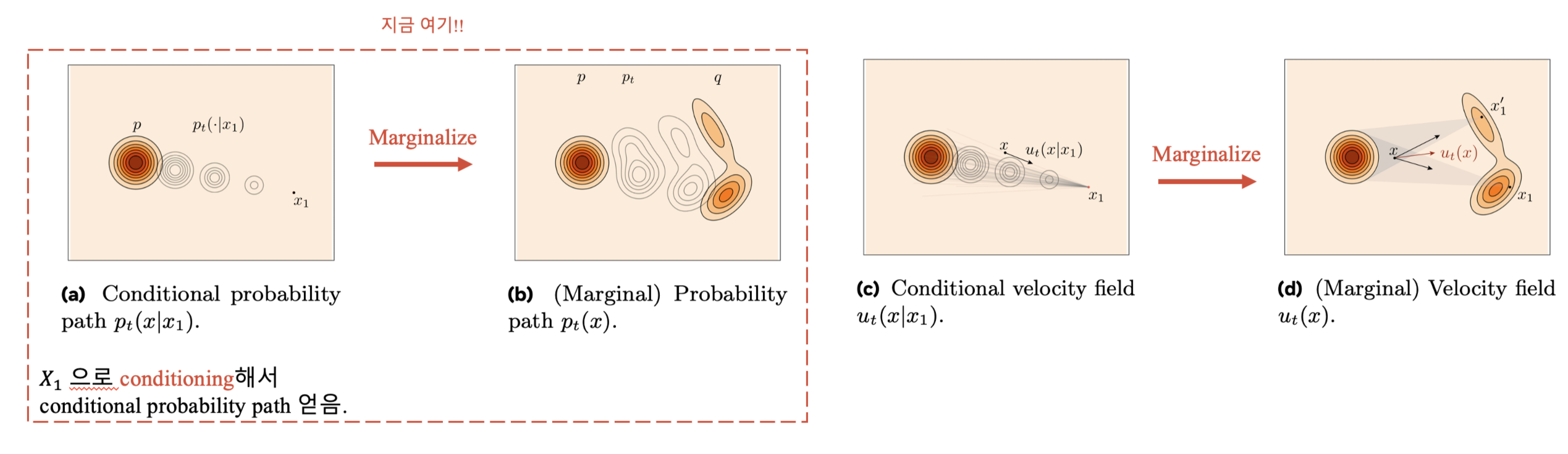
4.3. Deriving generating velocity fields
한 줄 요약. 위에서 구한 marginal probability path를 이용해 \(p_t\)를 생성하는 velocity field \(u_t\)를 유도 할수 있습니다.
Conditional velocity field \(u_t(x|x_1)\) 는 다음을 만족합니다.
\[u_t(\cdot|x_1) \quad \text{generates} \quad p_{t|1}(\cdot|x_1)\]이를 이용해 marginal velocity field 는 다음과 같이 계산됩니다. (Bayes’ Rule 사용)
\[u_t(x) = \int u_t(x|x_1) \color{red} p_{1|t}(x_1|x) \color{black} dx_1.\]- \(\color{red} p_{1|t}(x_1|x)\)를 현재 sample \(x\)로 conditioning 했을 때 target sample \(x_1\)의 posterior로 볼 수 있습니다.
혹은 Conditional expectation으로 볼 수 있습니다. (뒤에서 자주 나오는데, 초록색으로 표시하겠습니다.)
\(X_t \sim p_{t|1}(\cdot|x_1)\) 라 하면 다음을 얻습니다.
\[\color{green} u_t(x) = \mathbb{E}[u_t(X_t|X_1) \,|\, X_t = x]\]이는 \(X_t = x\)가 주어졌을 때, \(u_t(x)\)가 \(u_t(X_t|X_1)\)의 least-square approximation임을 의미합니다.
4.4. General Conditioning and the Marginalization Trick
위에서는 Conditioning을 single target sample \(X_1 = x_1\)에 대해서 했는데, 임의의 \(\text{RV}\)로 논의를 확장할 수 있습니다.
Marginal probability path :
\[p_t(x) = \int p_{t|Z}(x|z) p_Z(z) \, dz,\]이에 따른 marginal velocity field: \(u_t(x) = \int u_t(x|z) p_{Z|t}(z|x) \, dz = \color{green} \mathbb{E}[u_t(X_t | Z) \mid X_t = x].\)
\(\color{black}{\text{Theorem 3}}\) : Under some assumption, If \(u_t(x|z)\) generates \(p_t(\cdot|z)\),
then marginal velocity field \(u_t\) generates marginal probability path \(p_t\) !
(증명 생략)
4.5. Flow Matching loss
한 줄 요약. \(\nabla_\theta \mathcal{L}_{FM}(\theta) = \nabla_\theta \mathcal{L}_{CFM}(\theta).\)
자 지금까지 target velocity field \(u_t\), 이를 이용해 probability path, \(p_t\)를 만들었습니다만…
\(u_t^\theta\)를 학습하기 위해서는 tractable한 loss function을 정의해야 합니다.
Flow matching loss : \(\mathcal{L}_{\text{FM}}(\theta) = \mathbb{E}_{t, X_t \sim p_t} D(u_t(X_t), u_t^\theta(X_t)),\) 인데, target velocity \(u_t\)는 intractable!!
Conditional Flow Matching (CFM) loss : \(\mathcal{L}_{\text{CFM}}(\theta) = \mathbb{E}_{t, Z, X_t \sim p_t|Z(\cdot | Z)} D(u_t(X_t | Z), u_t^\theta(X_t)).\)
재밌는 사실은 두 loss에 대한 gradient가 같다는 것입니다.
\[\nabla_\theta \mathcal{L}_{FM}(\theta) = \nabla_\theta \mathcal{L}_{CFM}(\theta).\]Proposition1
사실 이는 Bregman divergences for learning conditional expectations에 따른 자연스러운 결과라고 합니다. 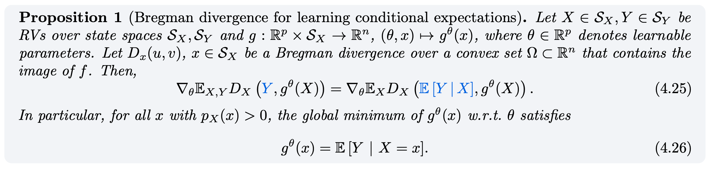
4.6. Solving conditional generation with conditional flows (핵심!)
자… 지금까지 우리는 flow model \(u_t^\theta\)을 학습하기 위해
- Conditional probability path 찾아서 B.C 과함께 marginal probability path 구함. (4.2)
- conditional probability path를 generate하는 Conditional velocity fields 유도. (4.3, 4.4)
- CFM loss 정의. (4.5)
이번 section에서는 1번과 2번, 즉, conditional probability paths and velocity fields를 design 하는 방법에 대해 살펴봅니다.
한 줄 요약. Conditional flow, \(\psi_t(\cdot|x_1)\) 를 이용해서 conditional path와 대응하는 velocity field 찾는 과정을 간단히!
B.C. 를 만족하는 flow model \(X_{t|1}\)를 정의하고
\(X_{t|1}\)를 미분하여 \(p_{t|1}(x|x_1) \quad \text{and} \quad u_t(x|x_1)\) 를 정의.
디테일하게 살펴봅시다.
- Conditional Flow Model, \(X_{t|1}\)
이며, 이때 Conditional flow, \(\psi_t(X_0|x_1) :[0, 1) \times \mathbb{R}^d \times \mathbb{R}^d \to \mathbb{R}^d\) 는 다음과 같이 정의됩니다.
\[\psi_t(x|x_1) = \begin{cases} x, & t = 0, \\ x_1, & t = 1. \end{cases}\]또한, push-forward formula를 이용해 \(X_{t|1}\) 의 probability density를 정의할 수 있습니다. (직접 사용되지는 않지만 B.C. 만족함을 보이는 데 사용)
\[p_{t|1}(x|x_1) := [\psi_t(\cdot|x_1)_\# \pi_{0|1}(\cdot|x_1)](x).\]- Conditional velocity field, \(u_t(x|x_1)\)
Flow와 velocity field의 동등성을 이용해 다음을 얻습니다.
\[u_t(x|x_1) = \frac{\partial}{\partial t} \psi_t(\psi_t^{-1}(x|x_1)|x_1).\]- Conditional Probability Path, \(p_{t|1}(x|x_1)\) :
위(4.3.) 에서 살펴본 것과 같이 \(u_t(x|x_1)\) 는 \(p_{t|1}(x|x_1)\) 를 generate합니다.
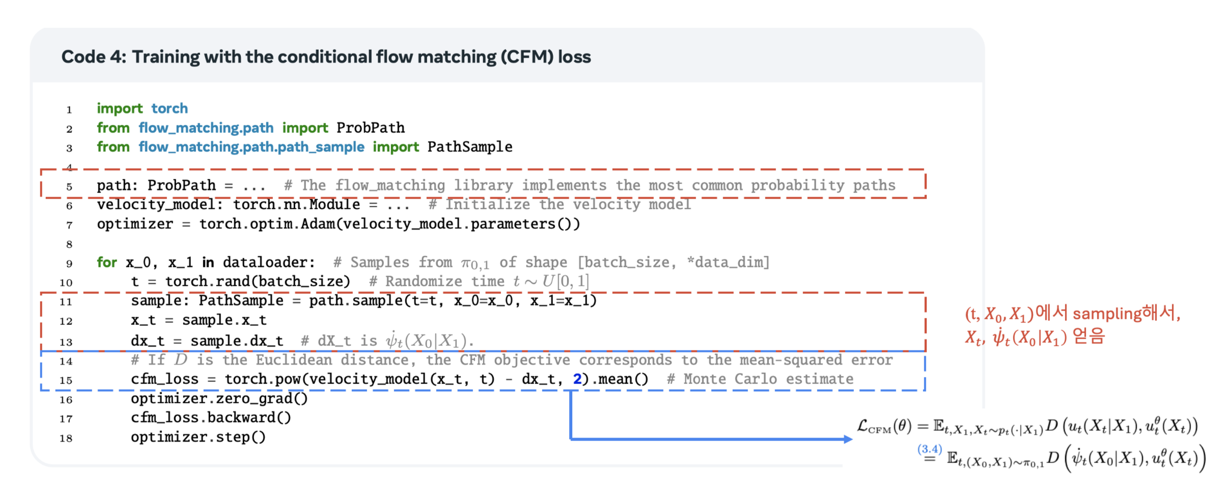
4.6.1. The Conditional Flow Matching loss, revisited (\(Z = X_1\))
\(Z = X_1\)으로 conditioning한 CFM loss는 conditional flow \(\psi_t(X_0|X_1)\)를 이용해 간단히 표현 가능합니다.
위에서 구한 CFM loss는 다음과 같습니다. (\(u_t(X_t | X_1) = \dot\psi_t \big( \psi_t^{-1}(\psi_t(X_0 | X_1) | X_1) \big) = \dot\psi_t(X_0 | X_1).\) 임을 이용해)
\[\begin{aligned} \mathcal{L}_{\text{CFM}}(\theta) &= \mathbb{E}_{t, X_1, X_t \sim p_t(\cdot | X_1)} D(u_t(X_t | X_1), u_t^\theta(X_t)) \\ &= \mathbb{E}_{t, (X_0, X_1) \sim \pi_{0,1}} D(\psi_t(X_0 | X_1), u_t^\theta(X_t)). \\ \end{aligned}\]이를 proposition1을 이용하면 loss가 최소가 되는 velocity는 다음과 같습니다. \(u_t(x) = \color{green}\mathbb{E}[\psi_t(X_0 | X_1) \mid X_t = x].\)
4.6.2. The Marginalization Trick for probability paths built from conditional flows
Conditional flows를 위한 새로운 Marginalization Trick을 소개합니다.
- Marginalization Trick은 Conditional Velocity Field \(u_t(x|x_1)\) 와 Probability Path \(p_{t|1}(x|x_1)\) 가 주어졌을 때, Marginal Path \(p_t(x)\)와 Marginal Velocity Field \(u_t(x)\)를 생성합니다.
- 이를 통해 Flow Matching 문제를 다양한 조건화 방식으로 해결할 수 있습니다.
4.6.3. Conditional flows with other conditions
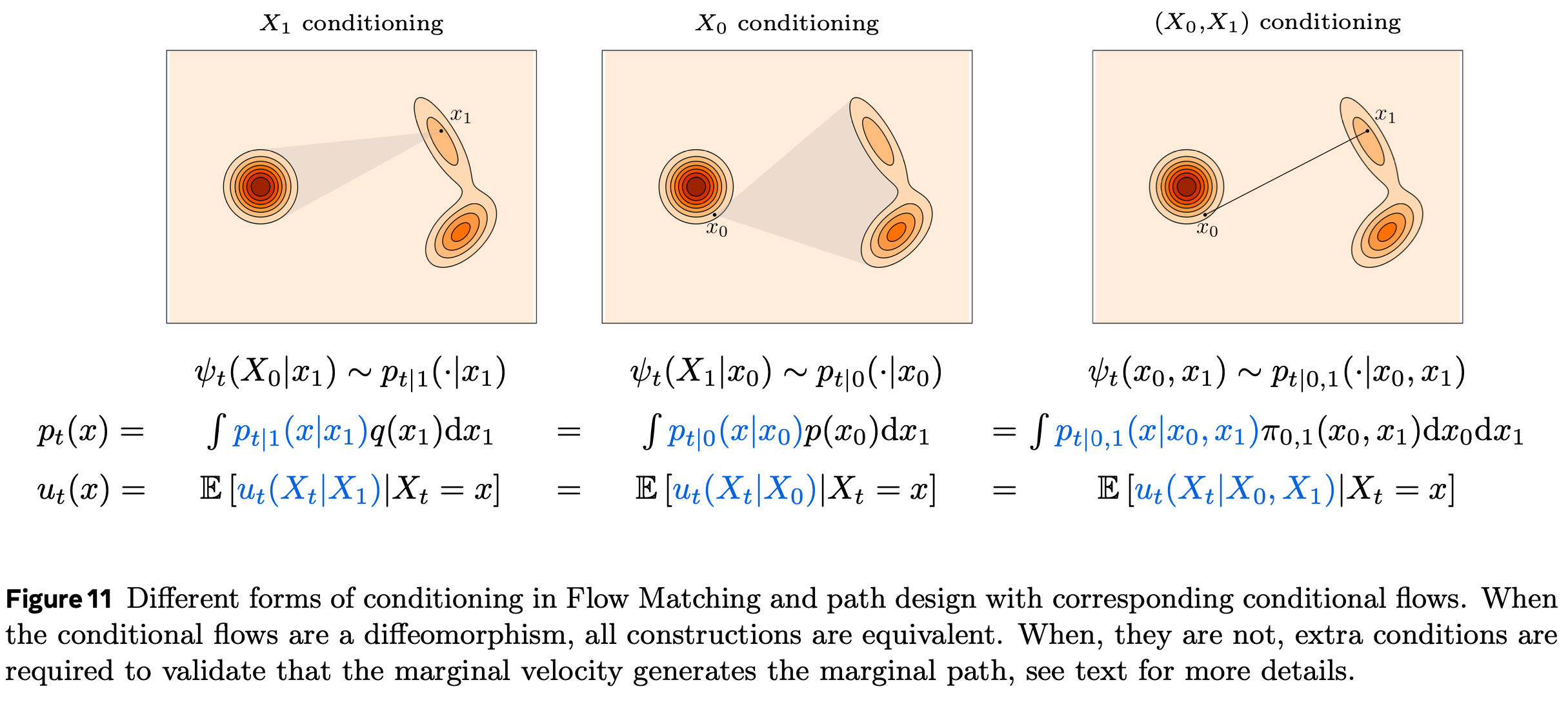
다양한 조건 \(Z = X_1, X_0, (X_0, X_1))\) 에 따른 conditional flow 설계를 다룹니다. (여러가지 choice가 있지만 flow가 diffeomorphism 이라면 모두 동일하다고 합니다.)
자 \(Z = (X_0, X_1)\)인 상황을 봅시다.
우리는 다음 조건을 만족하는 Conditional Probability Path \(p_{t|0,1}(x| x_0, x_1)\) 를 만들고 대응하는 velocity \(u_{t}(x| x_0, x_1)\)를 찾아야 합니다.
\[p_{0|0,1}(x|x_0, x_1) = \delta_{x_0}(x), \quad p_{1|0,1}(x|x_0, x_1) = \delta_{x_1}(x).\]\(X_{t|0,1} = \psi_t(x_0, x_1)\) 로 정의되는 Conditional flow,
\(\psi_t(X_0|x_1) :[0, 1) \times \mathbb{R}^d \times \mathbb{R}^d \to \mathbb{R}^d\) 는 다음을 만족합니다.
따라서 \(\psi(\cdot, x_1)\)은 \(\delta_{x_0} \to \delta_{x_1}\)으로 push 합니다.
- Conditional probability path 정의:
- B.C 를 만족하는 flow model 정의 :
- Conditional Velocity Field 정의 :
- Marginal Conditional Velocity Field 정의 :
4.7. Optimal Transport and linear conditional flow
그렇다면… useful conditional flow \(\psi_t(x|x_1)\) 는 어떻게 찾을 수 있을까요? 하나의 방법은 natural cost functional를 최소화 하는 것을 선택하는 것입니다. 유명한 예시 중 하나인 dynamic Optimal Transport problem에 따라 flow를 정의해봅시다.
\[(p_t^\star, u_t^\star) = \arg \min_{p_t, u_t} \int_0^1 \int \| u_t(x) \|^2 p_t(x) \, dx \, dt \quad \text{(Kinetic Energy)}\] \[\quad \text{s.t.} \quad p_0 = p, \, p_1 = q \quad \text{(interpolation)} \\ \quad \frac{\mathrm{d}}{\mathrm{d}t} p_t + \operatorname{div}(p_t u_t) = 0. \quad \text{(continuity equation)}\]위에서 구한 \((p_t^\star, u_t^\star)\)로 flow를 정의할 수 있습니다. \(\psi_t^\star(x) = t \phi(x) + (1 - t)x,\)
이는 OT displacement interpolant 라 불립니다. OT displacement interpolant도 R.V를 정의함으로써, Flow Matching problem을 해결할 수 있습니다.
\[X_t = \psi_t^\star(X_0) \sim p_t^\star \quad \text{when} \quad X_0 \sim p.\]Optimal Transport formulation은 직선 궤적을 장려하므로,
\[X_t = \psi_t^\star(X_0) = X_0 + t(\phi(X_0) - X_0),\]이를 열심히 계산해보면 (Euler-Lagrange equations)… 다음을 얻습니다.
\[\psi_t(x \mid x_1) = t x_1 + (1 - t)x.\]이로부터 얻을 수 있는 결론은 다음과 같습니다.
- Linear conditional flow가 Kinetic Energy를 minimize.
- Target \(q\)가 Single sample data point 라면 \(\psi_t(x \mid x_1) = t x_1 + (1 - t)x.\)는 Optimal Transport.
4.8. Affine conditional flows
이전 section 까지 Linear (conditional-OT) flow를 다뤘다면, 이번 section에서는 이를 더 일반화하여 affine conditional flow로 확장합니다.
\[\psi_t(x|x_1) = \alpha_t x_1 + \sigma_t x,\]이때, \((\alpha_t, \sigma_t)\)는 scheduler라 부릅니다.
\[u_t(x) =\color{green} \mathbb{E} \left[ \dot{\alpha}_t X_1 + \dot{\sigma}_t X_0 \mid X_t = x \right].\]또한 ~~한 조건 하에서는 위 marginal velocity \(u_t(x)\)가 \(p, q\)를 interpolate 함으로써 \(p_t\)를 generate 할 수 있다고 합니다.
Loss는 다음과 같습니다.
\[\mathcal{L}_{\text{CFM}}(\theta) = \mathbb{E}_{t, (X_0, X_1) \sim \pi_{0, 1}} D \left( \dot{\alpha}_t X_1 + \dot{\sigma}_t X_0, u_t^\theta(X_t) \right).\]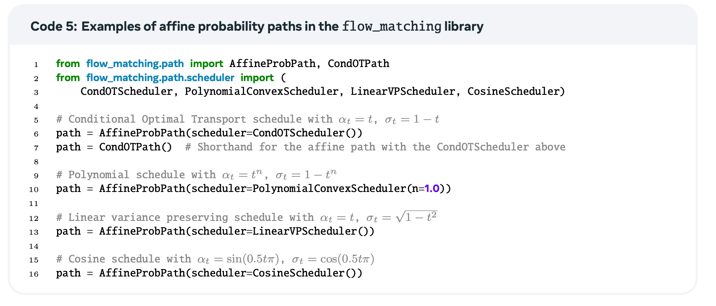
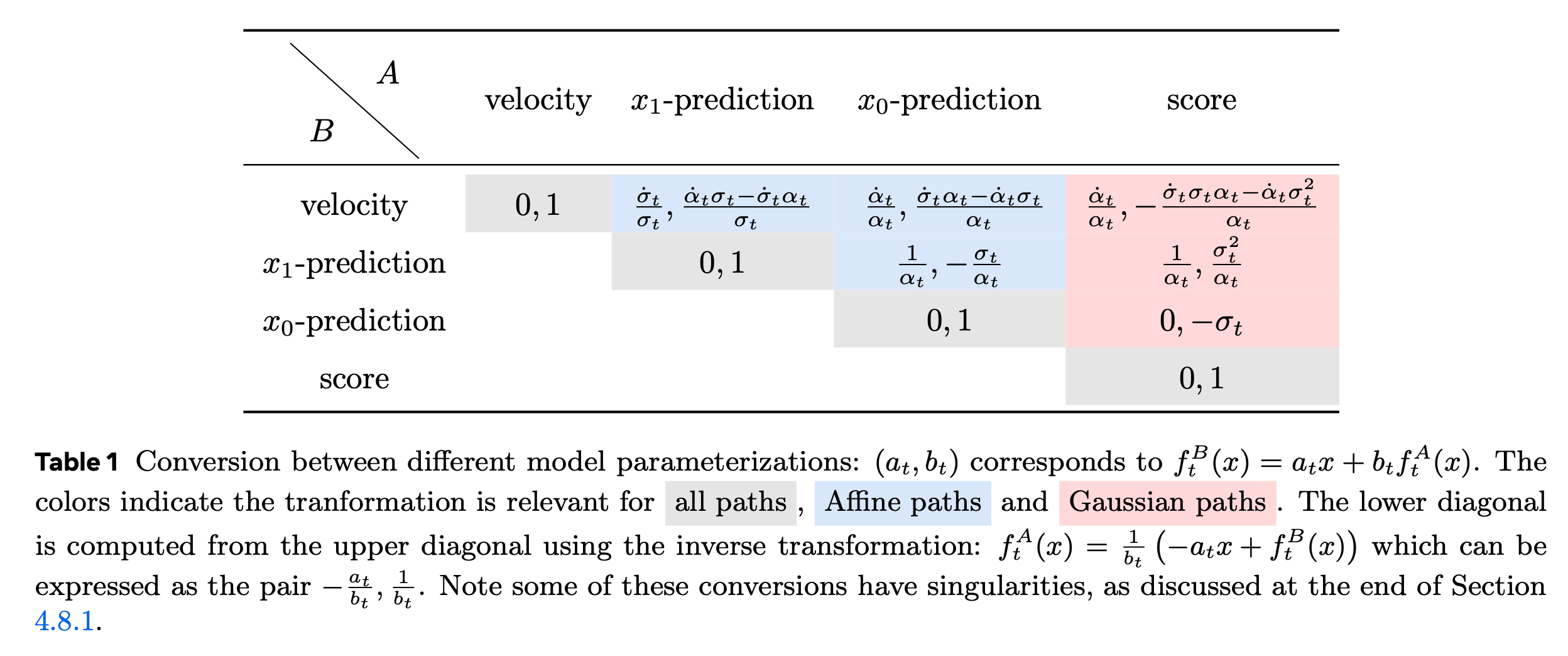
4.8.1. Velocity parameterizations
Affine case에서는 marginal velocity field \(u_t\)를 multiple parameterization할 수 있습니다.
\[X_t = \alpha_t X_1 + \sigma_t X_0 \iff X_1 = \frac{X_t - \sigma_t X_0}{\alpha_t} \iff X_0 = \frac{X_t - \alpha_t X_1}{\sigma_t}.\]이를 이용하면 다음을 얻을 수 있습니다.
\[\begin{aligned} \color{green} u_t(x) \color{black} &= \dot{\alpha}_t \color{blue} \mathbb{E} \left[ X_1 \mid X_t = x \right]\color{black} + \dot{\sigma}_t \color{red} \mathbb{E} \left[ X_0 \mid X_t = x \right] \color{black} \\ &= \frac{\dot{\sigma}_t}{\sigma_t} x + \left[ \dot{\alpha}_t - \alpha_t \frac{\dot{\sigma}_t}{\sigma_t} \right] \color{blue} \mathbb{E} \left[ X_1 \mid X_t = x \right]\color{black}\\ &= \frac{\dot{\alpha}_t}{\alpha_t} x + \left[ \dot{\sigma}_t - \sigma_t \frac{\dot{\alpha}_t}{\alpha_t} \right] \color{red}\mathbb{E} \left[ X_0 \mid X_t = x \right] \end{aligned}\]이를 deterministic function으로 다음과 같이 쓸 수 있습니다.
\[x_{1|t}(x) = \mathbb{E} \left[ X_1 \mid X_t = x \right] \quad \text{as the }\color{blue} x_1 \text{-prediction (target)} \color{black}\] \[x_{0|t}(x) = \mathbb{E} \left[ X_0 \mid X_t = x \right] \quad \text{as the } \color{red} x_0\text{-prediction (source)}\color{black}.\]any function \(g_t(x) := \mathbb{E} \left[ f_t(X_0, X_1) \mid X_t = x \right]\)에 대해 Matching loss는 다음과 같습니다.
\[\mathcal{L}_{\text{M}}(\theta) = \mathbb{E}_{t, X_t \sim p_t} D \left( g_t(X_t), g_t^\theta(X_t) \right).\]CFM loss와 비슷하게 Conditional Matching loss는 다음과 같습니다.
\[\mathcal{L}_{\text{CM}}(\theta) = \mathbb{E}_{t, (X_0, X_1) \sim \pi_{0,1}} D \left( f_t(X_0, X_1), g_t^\theta(X_t) \right).\]또한 이렇게 저렇게 증명해보면
\[\nabla_\theta \mathcal{L}_{\text{M}}(\theta) = \nabla_\theta \mathcal{L}_{\text{CM}}(\theta).\]를 얻을 수 있으며, 이때 loss를 최소화 하는 minimizer는 다음과 같습니다.
\[g_t^\theta(x) = \mathbb{E} \left[ f_t(X_0, X_1) \mid X_t = x \right].\]
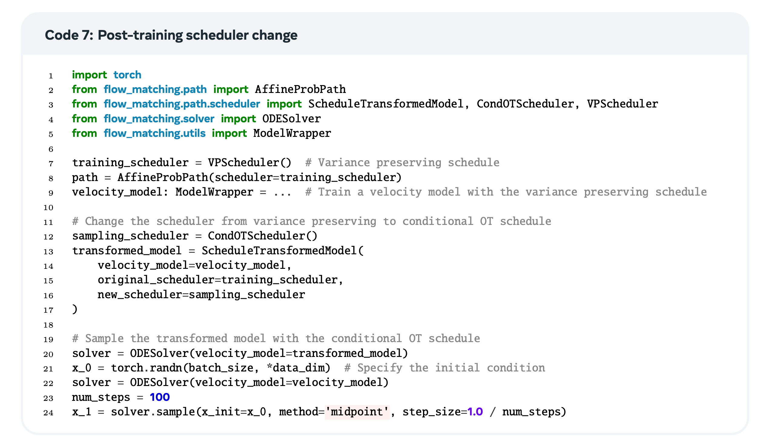
4.8.2. Post-training velocity scheduler change
Affine conditional flow는 marginal velocity field \(u_t\), (\((\alpha_t, \sigma_t)\), any \(\pi_{0, 1}\)) 에서 marginal velocity field \(\bar u_t\), (\((\bar\alpha_t, \bar\sigma_t)\), same \(\pi_{0, 1}\))으로 closed-form transformation을 제공합니다.
학습된 velocity field를 다른 scheduler로 바꾸어, 효율성을 높이거나, 생성 퀄리티를 높일 수 있습니다.
4.8.3. Gaussian paths
현재 가장 인기있는 affine probability path는
- Independent coupling : \(\pi_{0,1}(x_0, x_1) = p(x_0)q(x_1)\)
- Gaussian source distribution : \(p(x) = \mathcal{N}(x|0, \sigma^2 I)\)
이는 일반적인 diffusion model과 동일합니다. 예를 들어, Variance Preserving (VP) 와 Variance Exploding (VE)는 다음과 같이 정의됩니다.
- Variance Preserving : \(\alpha_t \equiv 1, \sigma_0 \gg 1, \sigma_1 = 0\)
- Variance Exploding : \(\alpha_t = e^{-\frac{1}{2} \beta_t}, \, \sigma_t = \sqrt{1 - e^{-\beta_t}}, \, \beta_0 \gg 1, \, \beta_1 = 0\)
또한 Gaussian 에서 중요한 quantity중 하나는 log probability의 gradient로 정의되는 Score가 있습니다.
\[\nabla \log p_{t|1}(x|x_1) = -\frac{1}{\sigma_t^2} (x - \alpha_t x_1)\]Marginal probability path의 Score는 다음과 같습니다.
\[\begin{aligned} \nabla \log p_t(x) &= \int \frac{\nabla p_{t|1}(x|x_1)q(x_1)}{p_t(x)} \, dx_1 \\ &= \int \nabla \log p_{t|1}(x|x_1) \frac{p_{t|1}(x|x_1)q(x_1)}{p_t(x)} \, dx_1 \\ &= \mathbb{E}\left[ \nabla \log p_{t|1}(X_t|X_1) \mid X_t = x \right] \\ &= \mathbb{E}\left[ -\frac{1}{\sigma_t^2} (X_t - \alpha_t X_1) \mid X_t = x \right] \\ &= \mathbb{E}\left[ -\frac{1}{\sigma_t} X_0 \mid X_t = x \right] \\ &= -\frac{1}{\sigma_t} x_{0|t}(x). \end{aligned}\]Diffusion model은 \(x_0\)-prediction, 혹은 noise-prediction입니다.
Gaussian path에서 velocity field는 다음과 같이 바꿔 쓸 수 있습니다.
\[\begin{aligned} u_t(x) &= \frac{\dot{\alpha}_t}{\alpha_t} x - \frac{\dot{\sigma}_t \sigma_t \alpha_t - \dot{\alpha}_t \sigma_t^2}{\alpha_t} \nabla \log p_t(x) \\ &= \nabla \left[ \frac{\dot{\alpha}_t}{2\alpha_t} \|x\|^2 - \frac{\dot{\sigma}_t \sigma_t \alpha_t - \dot{\alpha}_t \sigma_t^2}{\alpha_t} \log p_t(x) \right]. \end{aligned}\]여기서 \(u_t(x)\)는 gradient이므로 Kinetic Optimal 하다고 합니다.
4.9. Data couplings
지금까지 우리는 \((X_0, X_1) \sim \pi_{0,1}(X_0, X_1)\)에서 sampling 할 수 있다고 가정했는데,
- Independent samples : \(\pi_{0,1}(x_0, x_1) = p(x_0)q(x_1)\), 가장 간단한 형태로 지금까지 논의.
- Dependent samples : \((X_0, X_1) \sim \pi_{0,1}(X_0, X_1)\)
이 챕터에서는 Dependent sample의 몇 가지 예시를 봅니다.
4.9.1. Paired data
Inpainting 예시를 생각해봅시다. 우리의 목표는 masked-image \(x_0\) 를 대응하는 filled image \(x_1\) 로 mapping하는 과정을 학습하는 것입니다. 하지만 \(x_0\)에 대응하는 \(x_1\)위 개수는 많으므로, ill-defined problem 이라고 합니다.
이런 관찰에서, bridge 라는 방법이 제안되었습니다. 우리가 궁금한 \(\pi_{1|0}(x_1|x_0)\)은 sampling할 수 없지만, 반대 \(\pi_{0|1}(x_0|x_1)\) 는 구하기 쉽습니다. (단순히 마스킹 하면 되므로)
\[\pi_{0,1}(x_0, x_1) = \pi_{0|1}(x_0 | x_1) q(x_1).\]따라서 우리는 \((X_0, X_1)\) pair를 다음과 같은 과정을 통해 얻습니다.
- Draw \(X_1 \sim q\)
- Predefined randomized transformation, \(X_1\)으로부터 \(X_0\)얻음. 이때 어떤 condition을 맞추고, diversity를 늘리기 위해 \(\pi_{0|1}(x_0|x_1)\)에서 sampling할 때 noise를 추가한다고 합니다.
4.9.2. Multisample couplings
- \(X_0^{(i)} \sim p\), \(X_1^{(i)} \sim q\) sampling. (\(i \in [k]\))
- Construct \(\ \pi^k \in B_k \ \text{by} \ \pi^k := \arg \min_{\pi \in B_k} \mathbb{E}_{\pi} \left[ c(X_0^{(i)} - X_1^{(j)}) \right].\)
- Sample pair \((X_0^{(i)}, X_1^{(i)})\) uniformly at random, from \((X_0^{(i)}, X_1^{(j)})\) for which \(\pi^k(i,j) = 1\)
4.10 Conditional generation and guidance
4.10.1 Conditional models
Generative model에 guidance를 주는 가장 자연스러운 방법 중 하나는 conditional 분포 \(q(x_1 | y)\) 로부터 학습하는 것입니다.
Flow matching blueprint에따라 conditional target 분포 \(q(x_1 | y)\) 와 simple target 분포 \(p\) (e.g. Gaussian)를 고려하면, guided probability path는 다음과 같습니다.
\[p_{t|Y}(x|y) = \int p_{t|1}(x|x_1) q(x_1|y) \, dx_1.\]이때 guided probability path는 marginal endpoint 를 만족합니다. \(p_{0|Y}(\cdot|y) = p(\cdot), \, p_{1|Y}(\cdot|y) = q(\cdot|y).\)
guided velocity fields는 다음과 같습니다.
\[u_t(x|y) = \int u_t(x|x_1) p_{1|t,Y}(x_1|x,y) \, dx_1.\]열심히 계산해보면, \(u_t(x|y)\)가 \(p_{t|Y}(x|y)\) 를 generate하고, \(\text{FM/CFM}\) loss가 그대로라는 것을 보일 수 있습니다.
In practice, Guided marginal velocity field를 modeling할 때 single nueral net \(u_t^\theta\)를 학습한다고 합니다.
\[\mathcal{L}_{\mathrm{CFM}}(\theta) = \mathbb{E}_{t,(X_0,X_1,Y) \sim \pi_{0,1,Y}} D \left( \dot{\psi}_t(X_0|X_1), u_t^{\theta}(X_t|Y) \right).\]4.10.2 Classifier guidance and classifier-free guidance
Gaussian path로 학습된 flow는 velocity와 score function의 transformation을 이용해 CG, CFG를 사용할 수 있다고 합니다.
\[u_t(x|y) = a_t x + b_t \nabla \log p_{t|Y}(x|y)\]guided probability path에 Bayes’ rule을 적용하고, logarithm과 양변을 \(x\)에 대해 gradient를 취해주면 다음을 얻습니다.
\[\underbrace{\nabla \log p_{t|Y}(x|y)}_{\text{Conditional score}} = \underbrace{\nabla \log p_{Y|t}(y|x)}_{\text{Classifier}} + \underbrace{\nabla \log p_t(x)}_{\text{Unconditional score}}.\]이 관계에서 Classifier Guidance (CG)가 제안되었습니다. Unconditional model과 classifier를 이용해 conditional model에서 sampling하는 방법입니다. 이를 flow model을 사용해 나타내면 다음과 같습니다.
\[\tilde{u}_t^{\theta, \phi}(x|y) = a_t x + b_t \left( \nabla \log p_{Y|t}^\phi(y|x) + \nabla \log p_t^\theta(x) \right) = \underbrace{u_t^\theta(x)}_{\text{Uncond. Target } q(x) \text{ 에서 학습}} + b_t \nabla \underbrace{ \log p_{Y|t}^\phi(y|x)}_{\text{Classifier}},\]In practice, classifier, unconditional score는 따로 학습되므로 CG는 다음과 같이 표현해도 충분합니다.
\[\tilde{u}_t^{\theta, \phi}(x|y) = u_t^\theta(x) + b_t w \nabla \log p_{Y|t}^\phi(y|x),\]이후 연구에서는 위 식을 Re-arranging하여 Classifier-Free-Guidance (CFG)를 제안합니다.
\[\underbrace{\nabla \log p_{Y|t}(y|x)}_{\text{Classifier}} = \underbrace{\nabla \log p_{t|Y}(x|y)}_{\text{Conditional score}} - \underbrace{\nabla \log p_t(x)}_{\text{Unconditional score}}.\]이를 CG식에 넣으면
\[\tilde{u}_t^\theta(x|y) = (1 - w) u_t^\theta(x|\emptyset) + w u_t^\theta(x|y),\]하나의 모델 \({u}_t^\theta(x|y)\) 를 다음의 loss로 학습합니다.
\[\mathcal{L}_{\text{CFM}}(\theta) = \mathbb{E}_{t, \xi, (X_0, X_1, Y) \sim \pi_{0, 1, Y}} \left[ D\left( \psi_t(X_0 | X_1), u_t^\theta(X_t | ((1 - \xi) \cdot Y + \xi \cdot \emptyset)) \right) \right].\]