[Paper Reivew] Latent Diffsion Model(LDM)
LDM paper를 읽고 요약한 내용입니다.
CVPR 2022. [Paper] [Github]
Robin Rombach, Andreas Blattmann, Dominik Lorenz, Patrick Esser, Björn Ommer
Ludwig Maximilian University of Munich & IWR, Heidelberg University, Germany | Runway ML
20 Dec 2021
들어가며
이 포스팅은 High-Resolution Image Synthesis with Latent Diffusion Models를 읽고 공부한 내용을 담았습니다. 잘못된 내용이 있다면 댓글로 알려주세요 !
1. Abstract
Diffusion Model(DM)들이 좋은 성과를 내고 있지만, pixel space에서 동작하기 때문에 굉장히 많은 Resource(GPU, 시간,,,)가 필요하다. 이에 저자들은 pretrained autoencoder를 이용하여 확산 모델을 latent space에서 학습하여, 고해상도 이미지 생성을 훨씬 효율적으로 수행할 수 있음을 보였다. 또한 저자들은 cross-attention layer를 이용함으로써, DM을 여러가지 conditioning input에 대해 더 강력하고, 유연한 이미지 생성을 가능하게 했다.
2. Introduction
저자들의 주요 목표는 계산 비용을 크게 줄이면서도 기존 모델과 동등하거나 더 나은 성능을 달성하는 것이다.
저자들의 아이디어는 pixel space에서 학습된 DM을 분석하는 것에서 시작되었다. 다른 likelihood-based model들과 마찬가지로 학습은 크게 두 가지로 구분할 수 있다.
- Perceptual Compression: high-frequency detail을 제거하는 단계이다. 이때 semantic 정보는 거의 학습되지 않는다.
- Semantic Compression: 생성모델이 semantic한 정보를 학습하는 단계이다.
저자들은 Perceptually 동일하지만, 계산적으로 더 적합한 space를 찾는 것을 목표로 하여, 고해상도 이미지 생성을 위한 DM 모델을 학습하였다.
 Illustrating perceptual and semantic compression
따라서 저자들은 data space와 perceptually 동일한 lower dimensional space를 얻기 위해, autoencoder를 학습하였다. 이러한 방식을 사용해, 복잡성을 줄이고 더 효과적인 이미지 생성을 가능하게 하였다.
3. Method
DM이 관련없는 디테일들을 무시함으로써, 계산량을 줄이긴 하지만, 여전히 pixel space에서 계산 비용이 많이 발생한다. 이를 해결하기 위해 저자들은 학습단계에서 compressive와 generative learning 단계를 구분하는 것을 제안한다.
이러한 접근은 크게 3가지의 장점이 있다.
- 저차원 space에서 sampling 되므로 계산량을 크게 줄일 수 있다.
- UNet 구조로부터 inductive bias를 사용하므로, 공간 구조에 대해 효과적이다.
- General purpose compression model을 학습시키므로, latent space의 정보는 다양한 generative model 학습에 사용될 수 있으며, downstream application에도 활용 가능하다.
3.1. Perceptual Image Compression
저자들의 perceptual compression model은 perception loss와 patch-based adversarial objective의 combination으로 학습된 autoencoder로 구성된다.
자세히 보자면, 주어진 RGB 이미지 \(x \in \mathbb{R}^{H \times W \times 3}\)에 대해서 인코더 \(\mathcal{E}\)가 \(x\)를 latent representation으로 인코딩하고, \(z = \mathcal{E}(x)\) 디코더 \(\mathcal{D}\)가 latent \(z \in \mathbb{R}^{h \times w \times c}\)로부터 이미지를 재구성한다. \(\tilde{x} = \mathcal{D}(z) = \mathcal{D}(\mathcal{E}(x))\)
Autoencoding model의 전체 objective function은 다음과 같다.
\[\begin{equation} L_{\textrm{Autoencoder}} = \min_{\mathcal{E}, \mathcal{D}} \max_{\psi} \bigg( L_{\textrm{rec}} (x, \mathcal{D}(\mathcal{E}(x))) - L_{\textrm{adv}} (\mathcal{D}(\mathcal{E}(x))) + \log D_\psi (x) + L_{\textrm{reg}} (x; \mathcal{E}, \mathcal{D}) \bigg) \end{equation}\]3.2. Latent Diffusion Models
Diffusion Model의 loss function은 DDPM으로부터 다음과 같이 쓸 수 있다.
\[\begin{equation} L_{DM} = \mathbb{E}_{x, \epsilon \sim \mathcal{N} (0,1), t} \bigg[ \| \epsilon - \epsilon_\theta (x_t, t) \|_2^2 \bigg] \end{equation}\]이와 비교해 저자들이 제안한 Generative Modeling of Latent Representations은 인코더와 디코더를 이용하여 낮은 차원의 latent space에서 denoising 과정을 거치게 된다. 이때 loss function은 다음과 같이 정의된다.
\[\begin{equation} L_{LDM} := \mathbb{E}_{\mathcal{E}(x), \epsilon \sim \mathcal{N}(0,1), t} \bigg[ \| \epsilon - \epsilon_\theta (z_t, t) \|_2^2 \bigg] \end{equation}\]3.3. Conditioning Mechanisms
다른 생성형 모델과 마찬가지로, DM도 conditional distribution(\(p(z|y)\))을 모델링 하는 것이 가능하다. 이는 conditional denoising autoencoder \(\epsilon_\theta (z_t, t, y)\)로 구현되며, text, semantic map 혹은 다른 image-to-image translation task등 프로세스를 컨트롤 할 수 있다.
저자들은 UNet backbone을 cross-attention mechanism으로 보강하면서, 더 유연한 conditional 이미지 생성을 가능하게 한다. 다양한 modality로부터 \(y\)를 전처리하기 위해, domain specific encoder \(\tau_\theta\)를 도입한다. \(\tau_\theta (y) \in \mathbb{R}^{M \times d_\tau}\) 이는 이후 cross-attention layer에서 중간 layer에 매핑된다.
\[\begin{equation} \textrm{Attention}(Q, K, V) = \textrm{softmax}(\frac{QK^T}{\sqrt{d}}) \cdot V \end{equation}\]\(\begin{equation} Q = W_Q^{(i)} \cdot \phi_i (z_t), \quad K = W_K^{(i)} \cdot \tau_\theta (y), \quad V = W_V^{(i)} \cdot \tau_\epsilon (y) \end{equation}\) 따라서 image-condtioning pair를 기반으로, 다음 식을 이용해 condtional LDM을 학습할 수 있다.
\[\begin{equation} L_{LDM} := \mathbb{E}_{\mathcal{E} (x), y, \epsilon \sim \mathcal{N} (0, 1), t} \bigg[ \| \epsilon - \epsilon_\theta (z_t, t, \tau_\theta (y)) \|_2^2 \bigg] \end{equation}\]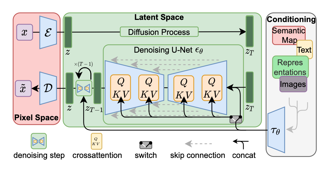
4. Experiments
저자들은 pixel based 모델과 저자들의 LDM을 training과 inference을 모두 비교한다. 저자들은 실험적으로 \(VQ\)-regularized latent space가 (초반엔 성능이 다소 안좋아 보이더라도) 때때로 더 나은 sample quality를 보임을 확인했다.
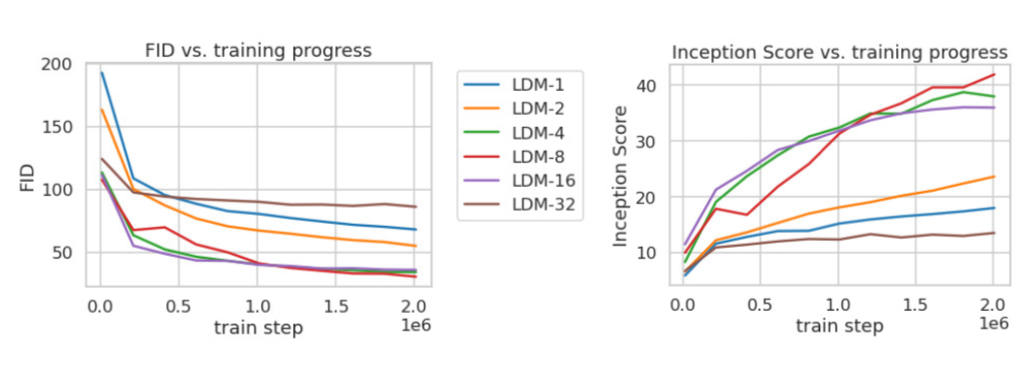
4.1. On Perceptual Compression Tradeoffs
저자들은 downsampling factor를 조절해가며, 최적의 latent space dimension을 찾고자 하였다. 실험적으로 \(f = 4, 8\)이 높은 퀄리티의 생성 결과를 나타내었다.
4.2. Image Generation with Latent Diffusion
저자들은 CelebA-HQ, FFHQ, LSUN-Churches and -Bedrooms 데이터셋을 이용하여, sample quality 와 data manifold의 coverage(FID, Precision-and-Recall) 를 측정하였으며, CelebA-HQ에서 SOTA FID 5.11을 달성했다고 한다.
또한 GAN-based 모델에 비해 Precision-and-Recall이 일관적으로 향상되었음을 확인하였다.
4.3. Conditional Latent Diffusion
Conditional Latent Diffusion은 이미지 생성 과정에서 조건(text, class label)을 반영하는 방식을 설명한다. 이 모델은 주어진 조건에 따라 이미지를 생성할 수 있으며, 특히 텍스트-이미지 생성 작업에서 뛰어난 성능을 보였다.
LDM은 cross-attention mechanism을 사용하여 주어진 condition을 latent space에 반영하고, 이를 기반으로 이미지의 특정 속성을 제어하며, 다양한 스타일이나 주제를 가진 이미지를 생성하는 데 유용한 것을 확인할 수 있다.
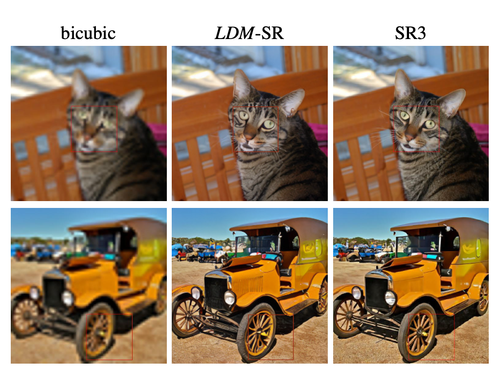
4.4 Super-Resolution with Latent Diffusion
4.5. Inpainting with Latent Diffusion

5. Limitations
latent space를 이용함으로써 LDM은 computational cost를 상당히 줄였음에도, sequential process 때문에 GAN 기반 이미지 생성보다는 느리다는 한계가 있다고 저자들은 말한다.
게다가, 매우 높은 수준의 이미지 생성을 위해서는 pixel space를 그대로 이용하는 것이 더 좋을 수 있다고 한다.
6. Conclusion
- Latent space에서 denoising을 하므로, computational cost를 상당히 줄였다.
- Latent space와 함께 Cross-attention conditioning mechanism layer를 사용함으로써, SOTA 성능을 달성할 수 있었다.
Reference
JiYeop Kim’s blog를 참고하여 작성하였습니다.